correct typos (#17)

* Add pypi workflow

* Fix wrong name

.github/workflows/python-publish.yml

@@ -0,0 +1,26 @@
+name: Upload Python Package
+
+on:
+  release:
+    types: [created]
+
+jobs:
+  deploy:
+    runs-on: ubuntu-latest
+    steps:
+    - uses: actions/checkout@v2
+    - name: Set up Python 3.6
+      uses: actions/setup-python@v2
+      with:
+        python-version: '3.6'
+    - name: Install dependencies
+      run: |
+        python -m pip install --upgrade pip
+        pip install setuptools wheel twine
+    - name: Build and publish
+      env:
+        TWINE_USERNAME: ${{ secrets.PYPI_USERNAME }}
+        TWINE_PASSWORD: ${{ secrets.PYPI_PASSWORD }}
+      run: |
+        python setup.py bdist_wheel
+        twine upload dist/*

.gitignore

@@ -1,10 +1,133 @@
-*.csv
-*.log
-*.pickle
-*.mp4
+# folders
+.vscode/
+.pytest_cache/
+result/
 
-.cache/
-.eggs/
+# Byte-compiled / optimized / DLL files
 __pycache__/
-.pytest_cache
-cache/
+*.py[cod]
+*$py.class
+
+# C extensions
+*.so
+
+# Distribution / packaging
+.Python
+build/
+develop-eggs/
+dist/
+downloads/
+eggs/
+.eggs/
+lib/
+lib64/
+parts/
+sdist/
+var/
+wheels/
+pip-wheel-metadata/
+share/python-wheels/
+*.egg-info/
+.installed.cfg
+*.egg
+MANIFEST
+
+# PyInstaller
+#  Usually these files are written by a python script from a template
+#  before PyInstaller builds the exe, so as to inject date/other infos into it.
+*.manifest
+*.spec
+
+# Installer logs
+pip-log.txt
+pip-delete-this-directory.txt
+
+# Unit test / coverage reports
+htmlcov/
+.tox/
+.nox/
+.coverage
+.coverage.*
+.cache
+nosetests.xml
+coverage.xml
+*.cover
+*.py,cover
+.hypothesis/
+.pytest_cache/
+
+# Translations
+*.mo
+*.pot
+
+# Django stuff:
+*.log
+local_settings.py
+db.sqlite3
+db.sqlite3-journal
+
+# Flask stuff:
+instance/
+.webassets-cache
+
+# Scrapy stuff:
+.scrapy
+
+# Sphinx documentation
+docs/_build/
+
+# PyBuilder
+target/
+
+# Jupyter Notebook
+.ipynb_checkpoints
+
+# IPython
+profile_default/
+ipython_config.py
+
+# pyenv
+.python-version
+
+# pipenv
+#   According to pypa/pipenv#598, it is recommended to include Pipfile.lock in version control.
+#   However, in case of collaboration, if having platform-specific dependencies or dependencies
+#   having no cross-platform support, pipenv may install dependencies that don't work, or not
+#   install all needed dependencies.
+#Pipfile.lock
+
+# PEP 582; used by e.g. github.com/David-OConnor/pyflow
+__pypackages__/
+
+# Celery stuff
+celerybeat-schedule
+celerybeat.pid
+
+# SageMath parsed files
+*.sage.py
+
+# Environments
+.env
+.venv
+venv/
+ENV/
+env.bak/
+venv.bak/
+
+# Spyder project settings
+.spyderproject
+.spyproject
+
+# Rope project settings
+.ropeproject
+
+# mkdocs documentation
+/site
+
+# mypy
+.mypy_cache/
+.dmypy.json
+dmypy.json
+
+# Pyre type checker
+.pyre/

.travis.yml

@@ -0,0 +1,14 @@
+language: python
+
+python:
+  - 3.7
+
+install:
+  - pip install --upgrade pip setuptools wheel
+  - pip install coveralls
+
+script:
+  - coverage run --source=PythonLinearNonlinearControl setup.py pytest
+
+after_success:
+  - coveralls

Environments.md

@@ -0,0 +1,68 @@
+# Enviroments
+
+| Name | Linear | Nonlinear | State Size | Input size |
+|:----------|:---------------:|:----------------:|:----------------:|:----------------:|
+| First Order Lag System | ✓ | x | 4 | 2 | 
+| Two wheeled System (Constant Goal) | x | ✓ | 3 | 2 | 
+| Two wheeled System (Moving Goal) (Coming soon) | x | ✓ | 3 | 2 | 
+| Cartpole (Swing up) | x | ✓ | 4 | 1 | 
+| Nonlinear Sample System Env | x | ✓ | 2 | 1 | 
+
+
+## [FistOrderLagEnv](PythonLinearNonlinearControl/envs/first_order_lag.py)
+
+### System equation.
+
+<img src="assets/firstorderlag.png" width="550">
+
+You can set arbinatry time constant, tau. The default is 0.63 s
+
+### Cost.
+
+<img src="assets/quadratic_score.png" width="300">
+
+Q = diag[1., 1., 1., 1.], 
+R = diag[1., 1.]
+
+X_g denote the goal states.
+
+## [TwoWheeledEnv](PythonLinearNonlinearControl/envs/two_wheeled.py)
+
+### System equation.
+
+<img src="assets/twowheeled.png" width="300">
+
+### Cost.
+
+<img src="assets/quadratic_score.png" width="300">
+
+Q = diag[5., 5., 1.], 
+R = diag[0.1, 0.1]
+
+X_g denote the goal states.
+
+## [CatpoleEnv (Swing up)](PythonLinearNonlinearControl/envs/cartpole.py)
+
+## System equation.
+
+<img src="assets/cartpole.png" width="600">
+
+You can set arbinatry parameters, mc, mp, l and g. 
+
+Default settings are as follows:
+
+mc = 1, mp = 0.2, l = 0.5, g = 9.81
+
+### Cost.
+
+<img src="assets/cartpole_score.png" width="300">
+
+## [Nonlinear Sample System Env](PythonLinearNonlinearControl/envs/nonlinear_sample_system.py)
+
+## System equation.
+
+<img src="assets/nonlinear_sample_system.png" width="400">
+
+### Cost.
+
+<img src="assets/nonlinear_sample_system_score.png" width="400">

PythonLinearNonlinearControl/common/utils.py

@@ -0,0 +1,147 @@
+import numpy as np
+
+
+def rotate_pos(pos, angle):
+    """ Transformation the coordinate in the angle
+
+    Args:
+        pos (numpy.ndarray): local state, shape(data_size, 2) 
+        angle (float): rotate angle, in radians
+    Returns:
+        rotated_pos (numpy.ndarray): shape(data_size, 2)
+    """
+    rot_mat = np.array([[np.cos(angle), -np.sin(angle)],
+                        [np.sin(angle), np.cos(angle)]])
+
+    return np.dot(pos, rot_mat.T)
+
+
+def fit_angle_in_range(angles, min_angle=-np.pi, max_angle=np.pi):
+    """ Check angle range and correct the range
+
+    Args:
+        angle (numpy.ndarray): in radians
+        min_angle (float): maximum of range in radians, default -pi
+        max_angle (float): minimum of range in radians, default pi
+    Returns: 
+        fitted_angle (numpy.ndarray): range angle in radians
+    """
+    if max_angle < min_angle:
+        raise ValueError("max angle must be greater than min angle")
+    if (max_angle - min_angle) < 2.0 * np.pi:
+        raise ValueError("difference between max_angle \
+                          and min_angle must be greater than 2.0 * pi")
+
+    output = np.array(angles)
+    output_shape = output.shape
+
+    output = output.flatten()
+    output -= min_angle
+    output %= 2 * np.pi
+    output += 2 * np.pi
+    output %= 2 * np.pi
+    output += min_angle
+
+    output = np.minimum(max_angle, np.maximum(min_angle, output))
+    return output.reshape(output_shape)
+
+
+def update_state_with_Runge_Kutta(state, u, functions, dt=0.01, batch=True):
+    """ update state in Runge Kutta methods
+    Args:
+        state (array-like): state of system
+        u (array-like): input of system
+        functions (list): update function of each state,
+            each function will be called like func(state, u)
+            We expect that this function returns differential of each state 
+        dt (float): float in seconds
+        batch (bool): state and u is given by batch or not
+
+    Returns:
+        next_state (np.array): next state of system
+
+    Notes:
+        sample of function is as follows:
+
+        def func_x(self, x_1, x_2, u):
+            x_dot = (1. - x_1**2 - x_2**2) * x_2 - x_1 + u
+            return x_dot
+
+        Note that the function return x_dot.
+    """
+    if not batch:
+        state_size = len(state)
+        assert state_size == len(functions), \
+            "Invalid functions length, You need to give the state size functions"
+
+        k0 = np.zeros(state_size)
+        k1 = np.zeros(state_size)
+        k2 = np.zeros(state_size)
+        k3 = np.zeros(state_size)
+
+        for i, func in enumerate(functions):
+            k0[i] = dt * func(state, u)
+
+        for i, func in enumerate(functions):
+            k1[i] = dt * func(state + k0 / 2., u)
+
+        for i, func in enumerate(functions):
+            k2[i] = dt * func(state + k1 / 2., u)
+
+        for i, func in enumerate(functions):
+            k3[i] = dt * func(state + k2, u)
+
+        return state + (k0 + 2. * k1 + 2. * k2 + k3) / 6.
+
+    else:
+        batch_size, state_size = state.shape
+        assert state_size == len(functions), \
+            "Invalid functions length, You need to give the state size functions"
+
+        k0 = np.zeros((batch_size, state_size))
+        k1 = np.zeros((batch_size, state_size))
+        k2 = np.zeros((batch_size, state_size))
+        k3 = np.zeros((batch_size, state_size))
+
+        for i, func in enumerate(functions):
+            k0[:, i] = dt * func(state, u)
+
+        for i, func in enumerate(functions):
+            k1[:, i] = dt * func(state + k0 / 2., u)
+
+        for i, func in enumerate(functions):
+            k2[:, i] = dt * func(state + k1 / 2., u)
+
+        for i, func in enumerate(functions):
+            k3[:, i] = dt * func(state + k2, u)
+
+        return state + (k0 + 2. * k1 + 2. * k2 + k3) / 6.
+
+
+def line_search(grad, sol, compute_eval_val,
+                init_alpha=0.001, max_iter=100, update_ratio=1.):
+    """ line search
+    Args:
+        grad (numpy.ndarray): gradient
+        sol (numpy.ndarray): sol
+        compute_eval_val (numpy.ndarray): function to compute evaluation value
+
+    Returns: 
+        alpha (float): result of line search 
+    """
+    assert grad.shape == sol.shape
+    base_val = np.inf
+    alpha = init_alpha
+    original_sol = sol.copy()
+
+    for _ in range(max_iter):
+        updated_sol = original_sol - alpha * grad
+        eval_val = compute_eval_val(updated_sol)
+
+        if eval_val < base_val:
+            alpha += init_alpha * update_ratio
+            base_val = eval_val
+        else:
+            break
+
+    return alpha

PythonLinearNonlinearControl/configs/__init__.py

@@ -0,0 +1,6 @@
+from PythonLinearNonlinearControl.configs.cartpole \
+    import CartPoleConfigModule  # NOQA
+from PythonLinearNonlinearControl.configs.first_order_lag \
+    import FirstOrderLagConfigModule  # NOQA
+from PythonLinearNonlinearControl.configs.two_wheeled \
+    import TwoWheeledConfigModule  # NOQA

PythonLinearNonlinearControl/configs/cartpole.py

@@ -0,0 +1,258 @@
+import numpy as np
+
+
+class CartPoleConfigModule():
+    # parameters
+    ENV_NAME = "CartPole-v0"
+    PLANNER_TYPE = "Const"
+    TYPE = "Nonlinear"
+    TASK_HORIZON = 500
+    PRED_LEN = 50
+    STATE_SIZE = 4
+    INPUT_SIZE = 1
+    DT = 0.02
+    # cost parameters
+    R = np.diag([0.01])  # 0.01 is worked for MPPI and CEM and MPPIWilliams
+    # 1. is worked for iLQR
+    TERMINAL_WEIGHT = 1.
+    Q = None
+    Sf = None
+    # bounds
+    INPUT_LOWER_BOUND = np.array([-3.])
+    INPUT_UPPER_BOUND = np.array([3.])
+    # parameters
+    MP = 0.2
+    MC = 1.
+    L = 0.5
+    G = 9.81
+    CART_SIZE = (0.15, 0.1)
+
+    def __init__(self):
+        """ 
+        """
+        # opt configs
+        self.opt_config = {
+            "Random": {
+                "popsize": 5000
+            },
+            "CEM": {
+                "popsize": 500,
+                "num_elites": 50,
+                "max_iters": 15,
+                "alpha": 0.3,
+                "init_var": 9.,
+                "threshold": 0.001
+            },
+            "MPPI": {
+                "beta": 0.6,
+                "popsize": 5000,
+                "kappa": 0.9,
+                "noise_sigma": 0.5,
+            },
+            "MPPIWilliams": {
+                "popsize": 5000,
+                "lambda": 1.,
+                "noise_sigma": 0.9,
+            },
+            "iLQR": {
+                "max_iter": 500,
+                "init_mu": 1.,
+                "mu_min": 1e-6,
+                "mu_max": 1e10,
+                "init_delta": 2.,
+                "threshold": 1e-6,
+            },
+            "DDP": {
+                "max_iter": 500,
+                "init_mu": 1.,
+                "mu_min": 1e-6,
+                "mu_max": 1e10,
+                "init_delta": 2.,
+                "threshold": 1e-6,
+            },
+            "NMPC-CGMRES": {
+            },
+            "NMPC-Newton": {
+            },
+        }
+
+    @staticmethod
+    def input_cost_fn(u):
+        """ input cost functions
+
+        Args:
+            u (numpy.ndarray): input, shape(pred_len, input_size)
+                or shape(pop_size, pred_len, input_size)
+        Returns:
+            cost (numpy.ndarray): cost of input, shape(pred_len, input_size) or
+                shape(pop_size, pred_len, input_size)
+        """
+        return (u**2) * np.diag(CartPoleConfigModule.R)
+
+    @staticmethod
+    def state_cost_fn(x, g_x):
+        """ state cost function
+
+        Args:
+            x (numpy.ndarray): state, shape(pred_len, state_size)
+                or shape(pop_size, pred_len, state_size)
+            g_x (numpy.ndarray): goal state, shape(pred_len, state_size)
+                or shape(pop_size, pred_len, state_size)
+        Returns:
+            cost (numpy.ndarray): cost of state, shape(pred_len, 1) or
+                shape(pop_size, pred_len, 1)
+        """
+
+        if len(x.shape) > 2:
+            return (6. * (x[:, :, 0]**2)
+                    + 12. * ((np.cos(x[:, :, 2]) + 1.)**2)
+                    + 0.1 * (x[:, :, 1]**2)
+                    + 0.1 * (x[:, :, 3]**2))[:, :, np.newaxis]
+
+        elif len(x.shape) > 1:
+            return (6. * (x[:, 0]**2)
+                    + 12. * ((np.cos(x[:, 2]) + 1.)**2)
+                    + 0.1 * (x[:, 1]**2)
+                    + 0.1 * (x[:, 3]**2))[:,  np.newaxis]
+
+        return 6. * (x[0]**2) \
+            + 12. * ((np.cos(x[2]) + 1.)**2) \
+            + 0.1 * (x[1]**2) \
+            + 0.1 * (x[3]**2)
+
+    @staticmethod
+    def terminal_state_cost_fn(terminal_x, terminal_g_x):
+        """
+
+        Args:
+            terminal_x (numpy.ndarray): terminal state,
+                shape(state_size, ) or shape(pop_size, state_size)
+            terminal_g_x (numpy.ndarray): terminal goal state,
+                shape(state_size, ) or shape(pop_size, state_size)
+        Returns:
+            cost (numpy.ndarray): cost of state, shape(pred_len, ) or
+                shape(pop_size, pred_len)
+        """
+
+        if len(terminal_x.shape) > 1:
+            return (6. * (terminal_x[:, 0]**2)
+                    + 12. * ((np.cos(terminal_x[:, 2]) + 1.)**2)
+                    + 0.1 * (terminal_x[:, 1]**2)
+                    + 0.1 * (terminal_x[:, 3]**2))[:, np.newaxis] \
+                * CartPoleConfigModule.TERMINAL_WEIGHT
+
+        return (6. * (terminal_x[0]**2)
+                + 12. * ((np.cos(terminal_x[2]) + 1.)**2)
+                + 0.1 * (terminal_x[1]**2)
+                + 0.1 * (terminal_x[3]**2)) \
+            * CartPoleConfigModule.TERMINAL_WEIGHT
+
+    @staticmethod
+    def gradient_cost_fn_state(x, g_x, terminal=False):
+        """ gradient of costs with respect to the state
+
+        Args:
+            x (numpy.ndarray): state, shape(pred_len, state_size)
+            g_x (numpy.ndarray): goal state, shape(pred_len, state_size)
+
+        Returns:
+            l_x (numpy.ndarray): gradient of cost, shape(pred_len, state_size)
+                or shape(1, state_size)
+        """
+        if not terminal:
+            cost_dx0 = 12. * x[:, 0]
+            cost_dx1 = 0.2 * x[:, 1]
+            cost_dx2 = 24. * (1 + np.cos(x[:, 2])) * -np.sin(x[:, 2])
+            cost_dx3 = 0.2 * x[:, 3]
+            cost_dx = np.stack((cost_dx0, cost_dx1,
+                                cost_dx2, cost_dx3), axis=1)
+            return cost_dx
+
+        cost_dx0 = 12. * x[0]
+        cost_dx1 = 0.2 * x[1]
+        cost_dx2 = 24. * (1 + np.cos(x[2])) * -np.sin(x[2])
+        cost_dx3 = 0.2 * x[3]
+        cost_dx = np.array([[cost_dx0, cost_dx1, cost_dx2, cost_dx3]])
+
+        return cost_dx * CartPoleConfigModule.TERMINAL_WEIGHT
+
+    @staticmethod
+    def gradient_cost_fn_input(x, u):
+        """ gradient of costs with respect to the input
+
+        Args:
+            x (numpy.ndarray): state, shape(pred_len, state_size)
+            u (numpy.ndarray): goal state, shape(pred_len, input_size)
+        Returns:
+            l_u (numpy.ndarray): gradient of cost, shape(pred_len, input_size)
+        """
+        return 2. * u * np.diag(CartPoleConfigModule.R)
+
+    @staticmethod
+    def hessian_cost_fn_state(x, g_x, terminal=False):
+        """ hessian costs with respect to the state
+
+        Args:
+            x (numpy.ndarray): state, shape(pred_len, state_size)
+            g_x (numpy.ndarray): goal state, shape(pred_len, state_size)
+        Returns:
+            l_xx (numpy.ndarray): gradient of cost,
+                shape(pred_len, state_size, state_size) or
+                shape(1, state_size, state_size) or
+        """
+        if not terminal:
+            (pred_len, state_size) = x.shape
+            hessian = np.eye(state_size)
+            hessian = np.tile(hessian, (pred_len, 1, 1))
+            hessian[:, 0, 0] = 12.
+            hessian[:, 1, 1] = 0.2
+            hessian[:, 2, 2] = 24. * -np.sin(x[:, 2]) \
+                * (-np.sin(x[:, 2])) \
+                + 24. * (1. + np.cos(x[:, 2])) \
+                * -np.cos(x[:, 2])
+            hessian[:, 3, 3] = 0.2
+
+            return hessian
+
+        state_size = len(x)
+        hessian = np.eye(state_size)
+        hessian[0, 0] = 12.
+        hessian[1, 1] = 0.2
+        hessian[2, 2] = 24. * -np.sin(x[2]) \
+            * (-np.sin(x[2])) \
+            + 24. * (1. + np.cos(x[2])) \
+            * -np.cos(x[2])
+        hessian[3, 3] = 0.2
+
+        return hessian[np.newaxis, :, :] * CartPoleConfigModule.TERMINAL_WEIGHT
+
+    @staticmethod
+    def hessian_cost_fn_input(x, u):
+        """ hessian costs with respect to the input
+
+        Args:
+            x (numpy.ndarray): state, shape(pred_len, state_size)
+            u (numpy.ndarray): goal state, shape(pred_len, input_size)
+        Returns:
+            l_uu (numpy.ndarray): gradient of cost,
+                shape(pred_len, input_size, input_size)
+        """
+        (pred_len, _) = u.shape
+
+        return np.tile(2.*CartPoleConfigModule.R, (pred_len, 1, 1))
+
+    @staticmethod
+    def hessian_cost_fn_input_state(x, u):
+        """ hessian costs with respect to the state and input
+
+        Args:
+            x (numpy.ndarray): state, shape(pred_len, state_size)
+            u (numpy.ndarray): goal state, shape(pred_len, input_size)
+        Returns:
+            l_ux (numpy.ndarray): gradient of cost ,
+                shape(pred_len, input_size, state_size)
+        """
+        (_, state_size) = x.shape
+        (pred_len, input_size) = u.shape
+
+        return np.zeros((pred_len, input_size, state_size))

PythonLinearNonlinearControl/configs/first_order_lag.py

@@ -0,0 +1,198 @@
+import numpy as np
+
+
+class FirstOrderLagConfigModule():
+    # parameters
+    ENV_NAME = "FirstOrderLag-v0"
+    TYPE = "Linear"
+    TASK_HORIZON = 1000
+    PRED_LEN = 50
+    STATE_SIZE = 4
+    INPUT_SIZE = 2
+    DT = 0.05
+    # cost parameters
+    R = np.eye(INPUT_SIZE)
+    Q = np.eye(STATE_SIZE)
+    Sf = np.eye(STATE_SIZE)
+    # bounds
+    INPUT_LOWER_BOUND = np.array([-0.5, -0.5])
+    INPUT_UPPER_BOUND = np.array([0.5, 0.5])
+    # DT_INPUT_LOWER_BOUND = np.array([-0.5 * DT, -0.5 * DT])
+    # DT_INPUT_UPPER_BOUND = np.array([0.25 * DT, 0.25 * DT])
+    DT_INPUT_LOWER_BOUND = None
+    DT_INPUT_UPPER_BOUND = None
+
+    def __init__(self):
+        """ 
+        """
+        # opt configs
+        self.opt_config = {
+            "Random": {
+                "popsize": 5000
+            },
+            "CEM": {
+                "popsize": 500,
+                "num_elites": 50,
+                "max_iters": 15,
+                "alpha": 0.3,
+                "init_var": 1.,
+                "threshold": 0.001
+            },
+            "MPPI": {
+                "beta": 0.6,
+                "popsize": 5000,
+                "kappa": 0.9,
+                "noise_sigma": 0.5,
+            },
+            "MPPIWilliams": {
+                "popsize": 5000,
+                "lambda": 1.,
+                "noise_sigma": 0.9,
+            },
+            "MPC": {
+            },
+            "iLQR": {
+                "max_iters": 500,
+                "init_mu": 1.,
+                "mu_min": 1e-6,
+                "mu_max": 1e10,
+                "init_delta": 2.,
+                "threshold": 1e-6,
+            },
+            "DDP": {
+                "max_iters": 500,
+                "init_mu": 1.,
+                "mu_min": 1e-6,
+                "mu_max": 1e10,
+                "init_delta": 2.,
+                "threshold": 1e-6,
+            },
+            "NMPC-CGMRES": {
+            },
+            "NMPC-Newton": {
+            },
+        }
+
+    @staticmethod
+    def input_cost_fn(u):
+        """ input cost functions
+        Args:
+            u (numpy.ndarray): input, shape(pred_len, input_size)
+                or shape(pop_size, pred_len, input_size)
+        Returns:
+            cost (numpy.ndarray): cost of input, shape(pred_len, input_size) or
+                shape(pop_size, pred_len, input_size)
+        """
+        return (u**2) * np.diag(FirstOrderLagConfigModule.R)
+
+    @staticmethod
+    def state_cost_fn(x, g_x):
+        """ state cost function
+        Args:
+            x (numpy.ndarray): state, shape(pred_len, state_size)
+                or shape(pop_size, pred_len, state_size)
+            g_x (numpy.ndarray): goal state, shape(pred_len, state_size)
+                or shape(pop_size, pred_len, state_size)
+        Returns:
+            cost (numpy.ndarray): cost of state, shape(pred_len, state_size) or
+                shape(pop_size, pred_len, state_size)
+        """
+        return ((x - g_x)**2) * np.diag(FirstOrderLagConfigModule.Q)
+
+    @staticmethod
+    def terminal_state_cost_fn(terminal_x, terminal_g_x):
+        """
+        Args:
+            terminal_x (numpy.ndarray): terminal state,
+                shape(state_size, ) or shape(pop_size, state_size)
+            terminal_g_x (numpy.ndarray): terminal goal state,
+                shape(state_size, ) or shape(pop_size, state_size)
+        Returns:
+            cost (numpy.ndarray): cost of state, shape(pred_len, ) or
+                shape(pop_size, pred_len)
+        """
+        return ((terminal_x - terminal_g_x)**2) \
+            * np.diag(FirstOrderLagConfigModule.Sf)
+
+    @staticmethod
+    def gradient_cost_fn_state(x, g_x, terminal=False):
+        """ gradient of costs with respect to the state
+
+        Args:
+            x (numpy.ndarray): state, shape(pred_len, state_size)
+            g_x (numpy.ndarray): goal state, shape(pred_len, state_size)
+
+        Returns:
+            l_x (numpy.ndarray): gradient of cost, shape(pred_len, state_size)
+                or shape(1, state_size)
+        """
+        if not terminal:
+            return 2. * (x - g_x) * np.diag(FirstOrderLagConfigModule.Q)
+
+        return (2. * (x - g_x)
+                * np.diag(FirstOrderLagConfigModule.Sf))[np.newaxis, :]
+
+    @staticmethod
+    def gradient_cost_fn_input(x, u):
+        """ gradient of costs with respect to the input
+
+        Args:
+            x (numpy.ndarray): state, shape(pred_len, state_size)
+            u (numpy.ndarray): goal state, shape(pred_len, input_size)
+
+        Returns:
+            l_u (numpy.ndarray): gradient of cost, shape(pred_len, input_size)
+        """
+        return 2. * u * np.diag(FirstOrderLagConfigModule.R)
+
+    @staticmethod
+    def hessian_cost_fn_state(x, g_x, terminal=False):
+        """ hessian costs with respect to the state
+
+        Args:
+            x (numpy.ndarray): state, shape(pred_len, state_size)
+            g_x (numpy.ndarray): goal state, shape(pred_len, state_size)
+
+        Returns:
+            l_xx (numpy.ndarray): gradient of cost,
+                shape(pred_len, state_size, state_size) or
+                shape(1, state_size, state_size) or
+        """
+        if not terminal:
+            (pred_len, _) = x.shape
+            return np.tile(2.*FirstOrderLagConfigModule.Q, (pred_len, 1, 1))
+
+        return np.tile(2.*FirstOrderLagConfigModule.Sf, (1, 1, 1))
+
+    @staticmethod
+    def hessian_cost_fn_input(x, u):
+        """ hessian costs with respect to the input
+
+        Args:
+            x (numpy.ndarray): state, shape(pred_len, state_size)
+            u (numpy.ndarray): goal state, shape(pred_len, input_size)
+
+        Returns:
+            l_uu (numpy.ndarray): gradient of cost,
+                shape(pred_len, input_size, input_size)
+        """
+        (pred_len, _) = u.shape
+
+        return np.tile(2.*FirstOrderLagConfigModule.R, (pred_len, 1, 1))
+
+    @staticmethod
+    def hessian_cost_fn_input_state(x, u):
+        """ hessian costs with respect to the state and input
+
+        Args:
+            x (numpy.ndarray): state, shape(pred_len, state_size)
+            u (numpy.ndarray): goal state, shape(pred_len, input_size)
+
+        Returns:
+            l_ux (numpy.ndarray): gradient of cost ,
+                shape(pred_len, input_size, state_size)
+        """
+        (_, state_size) = x.shape
+        (pred_len, input_size) = u.shape
+
+        return np.zeros((pred_len, input_size, state_size))

PythonLinearNonlinearControl/configs/make_configs.py

@@ -0,0 +1,23 @@
+from .first_order_lag import FirstOrderLagConfigModule
+from .two_wheeled import TwoWheeledConfigModule, TwoWheeledExtendConfigModule
+from .cartpole import CartPoleConfigModule
+from .nonlinear_sample_system import NonlinearSampleSystemConfigModule, NonlinearSampleSystemExtendConfigModule
+
+
+def make_config(args):
+    """
+    Returns:
+        config (ConfigModule class): configuration for the each env
+    """
+    if args.env == "FirstOrderLag":
+        return FirstOrderLagConfigModule()
+    elif args.env == "TwoWheeledConst" or args.env == "TwoWheeledTrack":
+        if args.controller_type == "NMPCCGMRES":
+            return TwoWheeledExtendConfigModule()
+        return TwoWheeledConfigModule()
+    elif args.env == "CartPole":
+        return CartPoleConfigModule()
+    elif args.env == "NonlinearSample":
+        if args.controller_type == "NMPCCGMRES":
+            return NonlinearSampleSystemExtendConfigModule()
+        return NonlinearSampleSystemConfigModule()

PythonLinearNonlinearControl/configs/nonlinear_sample_system.py

@@ -0,0 +1,353 @@
+import numpy as np
+
+
+class NonlinearSampleSystemConfigModule():
+    # parameters
+    ENV_NAME = "NonlinearSampleSystem-v0"
+    PLANNER_TYPE = "Const"
+    TYPE = "Nonlinear"
+    TASK_HORIZON = 2000
+    PRED_LEN = 10
+    STATE_SIZE = 2
+    INPUT_SIZE = 1
+    DT = 0.01
+    R = np.diag([1.])
+    Q = None
+    Sf = None
+    # bounds
+    INPUT_LOWER_BOUND = np.array([-0.5])
+    INPUT_UPPER_BOUND = np.array([0.5])
+
+    def __init__(self):
+        """
+        """
+        # opt configs
+        self.opt_config = {
+            "Random": {
+                "popsize": 5000
+            },
+            "CEM": {
+                "popsize": 500,
+                "num_elites": 50,
+                "max_iters": 15,
+                "alpha": 0.3,
+                "init_var": 9.,
+                "threshold": 0.001
+            },
+            "MPPI": {
+                "beta": 0.6,
+                "popsize": 5000,
+                "kappa": 0.9,
+                "noise_sigma": 0.5,
+            },
+            "MPPIWilliams": {
+                "popsize": 5000,
+                "lambda": 1.,
+                "noise_sigma": 0.9,
+            },
+            "iLQR": {
+                "max_iters": 500,
+                "init_mu": 1.,
+                "mu_min": 1e-6,
+                "mu_max": 1e10,
+                "init_delta": 2.,
+                "threshold": 1e-6,
+            },
+            "DDP": {
+                "max_iters": 500,
+                "init_mu": 1.,
+                "mu_min": 1e-6,
+                "mu_max": 1e10,
+                "init_delta": 2.,
+                "threshold": 1e-6,
+            },
+            "NMPC": {
+                "threshold": 0.01,
+                "max_iters": 5000,
+                "learning_rate": 0.01,
+                "optimizer_mode": "conjugate"
+            }
+        }
+
+    @staticmethod
+    def input_cost_fn(u):
+        """ input cost functions
+
+        Args:
+            u (numpy.ndarray): input, shape(pred_len, input_size)
+                or shape(pop_size, pred_len, input_size)
+        Returns:
+            cost (numpy.ndarray): cost of input, shape(pred_len, input_size) or
+                shape(pop_size, pred_len, input_size)
+        """
+        return (u**2) * np.diag(NonlinearSampleSystemConfigModule.R)
+
+    @staticmethod
+    def state_cost_fn(x, g_x):
+        """ state cost function
+
+        Args:
+            x (numpy.ndarray): state, shape(pred_len, state_size)
+                or shape(pop_size, pred_len, state_size)
+            g_x (numpy.ndarray): goal state, shape(pred_len, state_size)
+                or shape(pop_size, pred_len, state_size)
+        Returns:
+            cost (numpy.ndarray): cost of state, shape(pred_len, 1) or
+                shape(pop_size, pred_len, 1)
+        """
+
+        if len(x.shape) > 2:
+            return (0.5 * (x[:, :, 0]**2) +
+                    0.5 * (x[:, :, 1]**2))[:, :, np.newaxis]
+
+        elif len(x.shape) > 1:
+            return (0.5 * (x[:, 0]**2) + 0.5 * (x[:, 1]**2))[:, np.newaxis]
+
+        return 0.5 * (x[0]**2) + 0.5 * (x[1]**2)
+
+    @staticmethod
+    def terminal_state_cost_fn(terminal_x, terminal_g_x):
+        """
+
+        Args:
+            terminal_x (numpy.ndarray): terminal state,
+                shape(state_size, ) or shape(pop_size, state_size)
+            terminal_g_x (numpy.ndarray): terminal goal state,
+                shape(state_size, ) or shape(pop_size, state_size)
+        Returns:
+            cost (numpy.ndarray): cost of state, shape(pred_len, ) or
+                shape(pop_size, pred_len)
+        """
+
+        if len(terminal_x.shape) > 1:
+            return (0.5 * (terminal_x[:, 0]**2) +
+                    0.5 * (terminal_x[:, 1]**2))[:, np.newaxis]
+
+        return 0.5 * (terminal_x[0]**2) + 0.5 * (terminal_x[1]**2)
+
+    @staticmethod
+    def gradient_cost_fn_state(x, g_x, terminal=False):
+        """ gradient of costs with respect to the state
+
+        Args:
+            x (numpy.ndarray): state, shape(pred_len, state_size)
+            g_x (numpy.ndarray): goal state, shape(pred_len, state_size)
+
+        Returns:
+            l_x (numpy.ndarray): gradient of cost, shape(pred_len, state_size)
+                or shape(1, state_size)
+        """
+        if not terminal:
+            cost_dx0 = x[:, 0]
+            cost_dx1 = x[:, 1]
+            cost_dx = np.stack((cost_dx0, cost_dx1), axis=1)
+            return cost_dx
+
+        cost_dx0 = x[0]
+        cost_dx1 = x[1]
+        cost_dx = np.array([[cost_dx0, cost_dx1]])
+
+        return cost_dx
+
+    @staticmethod
+    def gradient_cost_fn_input(x, u):
+        """ gradient of costs with respect to the input
+
+        Args:
+            x (numpy.ndarray): state, shape(pred_len, state_size)
+            u (numpy.ndarray): goal state, shape(pred_len, input_size)
+        Returns:
+            l_u (numpy.ndarray): gradient of cost, shape(pred_len, input_size)
+        """
+        return 2. * u * np.diag(NonlinearSampleSystemConfigModule.R)
+
+    @staticmethod
+    def hessian_cost_fn_state(x, g_x, terminal=False):
+        """ hessian costs with respect to the state
+
+        Args:
+            x (numpy.ndarray): state, shape(pred_len, state_size)
+            g_x (numpy.ndarray): goal state, shape(pred_len, state_size)
+        Returns:
+            l_xx (numpy.ndarray): gradient of cost,
+                shape(pred_len, state_size, state_size) or
+                shape(1, state_size, state_size) or
+        """
+        if not terminal:
+            (pred_len, state_size) = x.shape
+            hessian = np.eye(state_size)
+            hessian = np.tile(hessian, (pred_len, 1, 1))
+            hessian[:, 0, 0] = 1.
+            hessian[:, 1, 1] = 1.
+
+            return hessian
+
+        state_size = len(x)
+        hessian = np.eye(state_size)
+        hessian[0, 0] = 1.
+        hessian[1, 1] = 1.
+
+        return hessian[np.newaxis, :, :]
+
+    @staticmethod
+    def hessian_cost_fn_input(x, u):
+        """ hessian costs with respect to the input
+
+        Args:
+            x (numpy.ndarray): state, shape(pred_len, state_size)
+            u (numpy.ndarray): goal state, shape(pred_len, input_size)
+        Returns:
+            l_uu (numpy.ndarray): gradient of cost,
+                shape(pred_len, input_size, input_size)
+        """
+        (pred_len, _) = u.shape
+
+        return np.tile(NonlinearSampleSystemConfigModule.R, (pred_len, 1, 1))
+
+    @staticmethod
+    def hessian_cost_fn_input_state(x, u):
+        """ hessian costs with respect to the state and input
+
+        Args:
+            x (numpy.ndarray): state, shape(pred_len, state_size)
+            u (numpy.ndarray): goal state, shape(pred_len, input_size)
+        Returns:
+            l_ux (numpy.ndarray): gradient of cost ,
+                shape(pred_len, input_size, state_size)
+        """
+        (_, state_size) = x.shape
+        (pred_len, input_size) = u.shape
+
+        return np.zeros((pred_len, input_size, state_size))
+
+    @staticmethod
+    def gradient_hamiltonian_input(x, lam, u, g_x):
+        """
+
+        Args:
+            x (numpy.ndarray): shape(pred_len+1, state_size)
+            lam (numpy.ndarray): shape(pred_len, state_size)
+            u (numpy.ndarray): shape(pred_len, input_size)
+            g_xs (numpy.ndarray): shape(pred_len, state_size)
+
+        Returns:
+            F (numpy.ndarray), shape(pred_len, input_size)
+        """
+        if len(x.shape) == 1:
+            input_size = u.shape[0]
+            F = np.zeros(input_size)
+            F[0] = u[0] + lam[1]
+
+            return F
+
+        elif len(x.shape) == 2:
+            pred_len, input_size = u.shape
+            F = np.zeros((pred_len, input_size))
+
+            for i in range(pred_len):
+                F[i, 0] = u[i, 0] + lam[i, 1]
+
+            return F
+
+        else:
+            raise NotImplementedError
+
+    @staticmethod
+    def gradient_hamiltonian_state(x, lam, u, g_x):
+        """
+        Args:
+            x (numpy.ndarray): shape(pred_len+1, state_size)
+            lam (numpy.ndarray): shape(pred_len, state_size)
+            u (numpy.ndarray): shape(pred_len, input_size)
+            g_xs (numpy.ndarray): shape(pred_len, state_size)
+
+        Returns:
+            lam_dot (numpy.ndarray), shape(state_size, )
+        """
+        if len(lam.shape) == 1:
+            state_size = lam.shape[0]
+            lam_dot = np.zeros(state_size)
+            lam_dot[0] = x[0] - (2. * x[0] * x[1] + 1.) * lam[1]
+            lam_dot[1] = x[1] + lam[0] + \
+                (-3. * (x[1]**2) - x[0]**2 + 1.) * lam[1]
+
+            return lam_dot
+
+        elif len(lam.shape) == 2:
+            pred_len, state_size = lam.shape
+            lam_dot = np.zeros((pred_len, state_size))
+
+            for i in range(pred_len):
+                lam_dot[i, 0] = x[i, 0] - \
+                    (2. * x[i, 0] * x[i, 1] + 1.) * lam[i, 1]
+                lam_dot[i, 1] = x[i, 1] + lam[i, 0] + \
+                    (-3. * (x[i, 1]**2) - x[i, 0]**2 + 1.) * lam[i, 1]
+
+            return lam_dot
+
+        else:
+            raise NotImplementedError
+
+
+class NonlinearSampleSystemExtendConfigModule(NonlinearSampleSystemConfigModule):
+    def __init__(self):
+        super().__init__()
+        self.opt_config = {
+            "NMPCCGMRES": {
+                "threshold": 1e-3,
+                "zeta": 100.,
+                "delta": 0.01,
+                "alpha": 0.5,
+                "tf": 1.,
+                "constraint": True
+            },
+            "NMPCNewton": {
+                "threshold": 1e-3,
+                "max_iteration": 500,
+                "learning_rate": 1e-3
+            }
+        }
+
+    @staticmethod
+    def gradient_hamiltonian_input_with_constraint(x, lam, u, g_x, dummy_u, raw):
+        """
+
+        Args:
+            x (numpy.ndarray): shape(pred_len+1, state_size)
+            lam (numpy.ndarray): shape(pred_len, state_size)
+            u (numpy.ndarray): shape(pred_len, input_size)
+            g_xs (numpy.ndarray): shape(pred_len, state_size)
+            dummy_u (numpy.ndarray): shape(pred_len, input_size)
+            raw (numpy.ndarray): shape(pred_len, input_size), Lagrangian for constraints
+
+        Returns:
+            F (numpy.ndarray), shape(pred_len, 3)
+        """
+        if len(x.shape) == 1:
+            vanilla_F = np.zeros(1)
+            extend_F = np.zeros(1)  # 1 is the same as input size
+            extend_C = np.zeros(1)
+
+            vanilla_F[0] = u[0] + lam[1] + 2. * raw[0] * u[0]
+            extend_F[0] = -0.01 + 2. * raw[0] * dummy_u[0]
+            extend_C[0] = u[0]**2 + dummy_u[0]**2 - \
+                NonlinearSampleSystemConfigModule.INPUT_LOWER_BOUND**2
+
+            F = np.concatenate([vanilla_F, extend_F, extend_C])
+
+        elif len(x.shape) == 2:
+            pred_len, _ = u.shape
+            vanilla_F = np.zeros((pred_len, 1))
+            extend_F = np.zeros((pred_len, 1))  # 1 is the same as input size
+            extend_C = np.zeros((pred_len, 1))
+
+            for i in range(pred_len):
+                vanilla_F[i, 0] = \
+                    u[i, 0] + lam[i, 1] + 2. * raw[i, 0] * u[i, 0]
+                extend_F[i, 0] = -0.01 + 2. * raw[i, 0] * dummy_u[i, 0]
+                extend_C[i, 0] = u[i, 0]**2 + dummy_u[i, 0]**2 - \
+                    NonlinearSampleSystemConfigModule.INPUT_LOWER_BOUND**2
+
+            F = np.concatenate([vanilla_F, extend_F, extend_C], axis=1)
+
+        return F

PythonLinearNonlinearControl/configs/two_wheeled.py

@@ -0,0 +1,408 @@
+import numpy as np
+from matplotlib.axes import Axes
+
+from ..plotters.plot_objs import square_with_angle, square
+from ..common.utils import fit_angle_in_range
+
+
+class TwoWheeledConfigModule():
+    # parameters
+    ENV_NAME = "TwoWheeled-v0"
+    TYPE = "Nonlinear"
+    N_AHEAD = 1
+    TASK_HORIZON = 1000
+    PRED_LEN = 20
+    STATE_SIZE = 3
+    INPUT_SIZE = 2
+    DT = 0.01
+    # cost parameters
+    # for Const goal
+    """
+    R = np.diag([0.1, 0.1])
+    Q = np.diag([1., 1., 0.01])
+    Sf = np.diag([5., 5., 1.])
+    """
+    # for track goal
+    """
+    R = np.diag([0.01, 0.01])
+    Q = np.diag([2.5, 2.5, 0.01])
+    Sf = np.diag([2.5, 2.5, 0.01])
+    """
+    # for track goal to NMPC
+    R = np.diag([1., 1.])
+    Q = np.diag([0.001, 0.001, 0.001])
+    Sf = np.diag([1., 1., 0.001])
+    # bounds
+    INPUT_LOWER_BOUND = np.array([-1.5, -3.14])
+    INPUT_UPPER_BOUND = np.array([1.5, 3.14])
+    # parameters
+    CAR_SIZE = 0.2
+    WHEELE_SIZE = (0.075, 0.015)
+
+    def __init__(self):
+        """ 
+        """
+        # opt configs
+        self.opt_config = {
+            "Random": {
+                "popsize": 5000
+            },
+            "CEM": {
+                "popsize": 500,
+                "num_elites": 50,
+                "max_iters": 15,
+                "alpha": 0.3,
+                "init_var": 1.,
+                "threshold": 0.001
+            },
+            "MPPI": {
+                "beta": 0.6,
+                "popsize": 5000,
+                "kappa": 0.9,
+                "noise_sigma": 0.5,
+            },
+            "MPPIWilliams": {
+                "popsize": 5000,
+                "lambda": 1,
+                "noise_sigma": 1.,
+            },
+            "iLQR": {
+                "max_iters": 500,
+                "init_mu": 1.,
+                "mu_min": 1e-6,
+                "mu_max": 1e10,
+                "init_delta": 2.,
+                "threshold": 1e-6,
+            },
+            "DDP": {
+                "max_iters": 500,
+                "init_mu": 1.,
+                "mu_min": 1e-6,
+                "mu_max": 1e10,
+                "init_delta": 2.,
+                "threshold": 1e-6,
+            },
+            "NMPC": {
+                "threshold": 0.01,
+                "max_iters": 5000,
+                "learning_rate": 0.01,
+                "optimizer_mode": "conjugate"
+            },
+            "NMPC-CGMRES": {
+            },
+            "NMPC-Newton": {
+            },
+        }
+
+    @staticmethod
+    def input_cost_fn(u):
+        """ input cost functions
+        Args:
+            u (numpy.ndarray): input, shape(pred_len, input_size)
+                or shape(pop_size, pred_len, input_size)
+        Returns:
+            cost (numpy.ndarray): cost of input, shape(pred_len, input_size) or
+                shape(pop_size, pred_len, input_size)
+        """
+        return (u**2) * np.diag(TwoWheeledConfigModule.R)
+
+    @staticmethod
+    def fit_diff_in_range(diff_x):
+        """ fit difference state in range(angle)
+
+        Args:
+            diff_x (numpy.ndarray): 
+                shape(pop_size, pred_len, state_size) or
+                shape(pred_len, state_size) or
+                shape(state_size, )
+        Returns:
+            fitted_diff_x (numpy.ndarray): same shape as diff_x
+        """
+        if len(diff_x.shape) == 3:
+            diff_x[:, :, -1] = fit_angle_in_range(diff_x[:, :, -1])
+        elif len(diff_x.shape) == 2:
+            diff_x[:, -1] = fit_angle_in_range(diff_x[:, -1])
+        elif len(diff_x.shape) == 1:
+            diff_x[-1] = fit_angle_in_range(diff_x[-1])
+
+        return diff_x
+
+    @staticmethod
+    def state_cost_fn(x, g_x):
+        """ state cost function
+        Args:
+            x (numpy.ndarray): state, shape(pred_len, state_size)
+                or shape(pop_size, pred_len, state_size)
+            g_x (numpy.ndarray): goal state, shape(pred_len, state_size)
+                or shape(pop_size, pred_len, state_size)
+        Returns:
+            cost (numpy.ndarray): cost of state, shape(pred_len, state_size) or
+                shape(pop_size, pred_len, state_size)
+        """
+        diff = TwoWheeledConfigModule.fit_diff_in_range(x - g_x)
+        return ((diff)**2) * np.diag(TwoWheeledConfigModule.Q)
+
+    @staticmethod
+    def terminal_state_cost_fn(terminal_x, terminal_g_x):
+        """
+        Args:
+            terminal_x (numpy.ndarray): terminal state,
+                shape(state_size, ) or shape(pop_size, state_size)
+            terminal_g_x (numpy.ndarray): terminal goal state,
+                shape(state_size, ) or shape(pop_size, state_size)
+        Returns:
+            cost (numpy.ndarray): cost of state, shape(pred_len, ) or
+                shape(pop_size, pred_len)
+        """
+        terminal_diff = TwoWheeledConfigModule.fit_diff_in_range(terminal_x
+                                                                 - terminal_g_x)
+
+        return ((terminal_diff)**2) * np.diag(TwoWheeledConfigModule.Sf)
+
+    @staticmethod
+    def gradient_cost_fn_state(x, g_x, terminal=False):
+        """ gradient of costs with respect to the state
+
+        Args:
+            x (numpy.ndarray): state, shape(pred_len, state_size)
+            g_x (numpy.ndarray): goal state, shape(pred_len, state_size)
+
+        Returns:
+            l_x (numpy.ndarray): gradient of cost, shape(pred_len, state_size)
+                or shape(1, state_size)
+        """
+        diff = TwoWheeledConfigModule.fit_diff_in_range(x - g_x)
+
+        if not terminal:
+            return 2. * (diff) * np.diag(TwoWheeledConfigModule.Q)
+
+        return (2. * (diff)
+                * np.diag(TwoWheeledConfigModule.Sf))[np.newaxis, :]
+
+    @staticmethod
+    def gradient_cost_fn_input(x, u):
+        """ gradient of costs with respect to the input
+
+        Args:
+            x (numpy.ndarray): state, shape(pred_len, state_size)
+            u (numpy.ndarray): goal state, shape(pred_len, input_size)
+
+        Returns:
+            l_u (numpy.ndarray): gradient of cost, shape(pred_len, input_size)
+        """
+        return 2. * u * np.diag(TwoWheeledConfigModule.R)
+
+    @staticmethod
+    def hessian_cost_fn_state(x, g_x, terminal=False):
+        """ hessian costs with respect to the state
+
+        Args:
+            x (numpy.ndarray): state, shape(pred_len, state_size)
+            g_x (numpy.ndarray): goal state, shape(pred_len, state_size)
+
+        Returns:
+            l_xx (numpy.ndarray): gradient of cost,
+                shape(pred_len, state_size, state_size) or
+                shape(1, state_size, state_size) or
+        """
+        if not terminal:
+            (pred_len, _) = x.shape
+            return np.tile(2.*TwoWheeledConfigModule.Q, (pred_len, 1, 1))
+
+        return np.tile(2.*TwoWheeledConfigModule.Sf, (1, 1, 1))
+
+    @staticmethod
+    def hessian_cost_fn_input(x, u):
+        """ hessian costs with respect to the input
+
+        Args:
+            x (numpy.ndarray): state, shape(pred_len, state_size)
+            u (numpy.ndarray): goal state, shape(pred_len, input_size)
+
+        Returns:
+            l_uu (numpy.ndarray): gradient of cost,
+                shape(pred_len, input_size, input_size)
+        """
+        (pred_len, _) = u.shape
+
+        return np.tile(2.*TwoWheeledConfigModule.R, (pred_len, 1, 1))
+
+    @staticmethod
+    def hessian_cost_fn_input_state(x, u):
+        """ hessian costs with respect to the state and input
+
+        Args:
+            x (numpy.ndarray): state, shape(pred_len, state_size)
+            u (numpy.ndarray): goal state, shape(pred_len, input_size)
+
+        Returns:
+            l_ux (numpy.ndarray): gradient of cost ,
+                shape(pred_len, input_size, state_size)
+        """
+        (_, state_size) = x.shape
+        (pred_len, input_size) = u.shape
+
+        return np.zeros((pred_len, input_size, state_size))
+
+    @staticmethod
+    def gradient_hamiltonian_input(x, lam, u, g_x):
+        """
+
+        Args:
+            x (numpy.ndarray): shape(pred_len+1, state_size)
+            lam (numpy.ndarray): shape(pred_len, state_size)
+            u (numpy.ndarray): shape(pred_len, input_size)
+            g_xs (numpy.ndarray): shape(pred_len, state_size)
+
+        Returns:
+            F (numpy.ndarray), shape(pred_len, input_size)
+        """
+        if len(x.shape) == 1:
+            input_size = u.shape[0]
+            F = np.zeros(input_size)
+            F[0] = u[0] * TwoWheeledConfigModule.R[0, 0] + \
+                lam[0] * np.cos(x[2]) + lam[1] * np.sin(x[2])
+            F[1] = u[1] * TwoWheeledConfigModule.R[1, 1] + lam[2]
+
+            return F
+
+        elif len(x.shape) == 2:
+            pred_len, input_size = u.shape
+            F = np.zeros((pred_len, input_size))
+
+            for i in range(pred_len):
+                F[i, 0] = u[i, 0] * TwoWheeledConfigModule.R[0, 0] + \
+                    lam[i, 0] * np.cos(x[i, 2]) + lam[i, 1] * np.sin(x[i, 2])
+                F[i, 1] = u[i, 1] * TwoWheeledConfigModule.R[1, 1] + lam[i, 2]
+
+            return F
+        else:
+            raise NotImplementedError
+
+    @staticmethod
+    def gradient_hamiltonian_state(x, lam, u, g_x):
+        """
+        Args:
+            x (numpy.ndarray): shape(pred_len+1, state_size)
+            lam (numpy.ndarray): shape(pred_len, state_size)
+            u (numpy.ndarray): shape(pred_len, input_size)
+            g_xs (numpy.ndarray): shape(pred_len, state_size)
+
+        Returns:
+            lam_dot (numpy.ndarray), shape(state_size, )
+        """
+        if len(lam.shape) == 1:
+            state_size = lam.shape[0]
+            lam_dot = np.zeros(state_size)
+            lam_dot[0] = \
+                (x[0] - g_x[0]) * TwoWheeledConfigModule.Q[0, 0]
+            lam_dot[1] = \
+                (x[1] - g_x[1]) * TwoWheeledConfigModule.Q[1, 1]
+
+            relative_angle = fit_angle_in_range(x[2] - g_x[2])
+            lam_dot[2] = \
+                relative_angle * TwoWheeledConfigModule.Q[2, 2] \
+                - lam[0] * u[0] * np.sin(x[2]) \
+                + lam[1] * u[0] * np.cos(x[2])
+
+            return lam_dot
+
+        elif len(lam.shape) == 2:
+            pred_len, state_size = lam.shape
+            lam_dot = np.zeros((pred_len, state_size))
+
+            for i in range(pred_len):
+                lam_dot[i, 0] = \
+                    (x[i, 0] - g_x[i, 0]) * TwoWheeledConfigModule.Q[0, 0]
+                lam_dot[i, 1] = \
+                    (x[i, 1] - g_x[i, 1]) * TwoWheeledConfigModule.Q[1, 1]
+
+                relative_angle = fit_angle_in_range(x[i, 2] - g_x[i, 2])
+                lam_dot[i, 2] = \
+                    relative_angle * TwoWheeledConfigModule.Q[2, 2] \
+                    - lam[i, 0] * u[i, 0] * np.sin(x[i, 2]) \
+                    + lam[i, 1] * u[i, 0] * np.cos(x[i, 2])
+
+            return lam_dot
+        else:
+            raise NotImplementedError
+
+
+class TwoWheeledExtendConfigModule(TwoWheeledConfigModule):
+    PRED_LEN = 20
+
+    def __init__(self):
+        super().__init__()
+        self.opt_config = {
+            "NMPCCGMRES": {
+                "threshold": 1e-3,
+                "zeta": 5.,
+                "delta": 0.01,
+                "alpha": 0.5,
+                "tf": 1.,
+                "constraint": True
+            },
+            "NMPCNewton": {
+                "threshold": 1e-3,
+                "max_iteration": 500,
+                "learning_rate": 1e-3
+            }
+        }
+
+    @staticmethod
+    def gradient_hamiltonian_input_with_constraint(x, lam, u, g_x, dummy_u, raw):
+        """
+
+        Args:
+            x (numpy.ndarray): shape(pred_len+1, state_size)
+            lam (numpy.ndarray): shape(pred_len, state_size)
+            u (numpy.ndarray): shape(pred_len, input_size)
+            g_xs (numpy.ndarray): shape(pred_len, state_size)
+            dummy_u (numpy.ndarray): shape(pred_len, input_size)
+            raw (numpy.ndarray): shape(pred_len, input_size), Lagrangian for constraints
+
+        Returns:
+            F (numpy.ndarray), shape(pred_len, 3)
+        """
+        if len(x.shape) == 1:
+            vanilla_F = np.zeros(2)
+            extend_F = np.zeros(2)  # 1 is the same as input size
+            extend_C = np.zeros(2)
+
+            vanilla_F[0] = u[0] + lam[0] * \
+                np.cos(x[2]) + lam[1] * np.sin(x[2]) + 2. * raw[0] * u[0]
+            vanilla_F[1] = u[1] + lam[2] + 2 * raw[1] * u[1]
+
+            extend_F[0] = -0.01 + 2. * raw[0] * dummy_u[0]
+            extend_F[1] = -0.01 + 2. * raw[1] * dummy_u[1]
+
+            extend_C[0] = u[0]**2 + dummy_u[0]**2 - \
+                TwoWheeledConfigModule.INPUT_LOWER_BOUND[0]**2
+            extend_C[1] = u[1]**2 + dummy_u[1]**2 - \
+                TwoWheeledConfigModule.INPUT_LOWER_BOUND[1]**2
+
+            F = np.concatenate([vanilla_F, extend_F, extend_C])
+
+        elif len(x.shape) == 2:
+            pred_len, _ = u.shape
+            vanilla_F = np.zeros((pred_len, 2))
+            extend_F = np.zeros((pred_len, 2))  # 1 is the same as input size
+            extend_C = np.zeros((pred_len, 2))
+
+            for i in range(pred_len):
+                vanilla_F[i, 0] = u[i, 0] + lam[i, 0] * \
+                    np.cos(x[i, 2]) + lam[i, 1] * \
+                    np.sin(x[i, 2]) + 2. * raw[i, 0] * u[i, 0]
+                vanilla_F[i, 1] = u[i, 1] + lam[i, 2] + 2 * raw[i, 1] * u[i, 1]
+
+                extend_F[i, 0] = -0.01 + 2. * raw[i, 0] * dummy_u[i, 0]
+                extend_F[i, 1] = -0.01 + 2. * raw[i, 1] * dummy_u[i, 1]
+
+                extend_C[i, 0] = u[i, 0]**2 + dummy_u[i, 0]**2 - \
+                    TwoWheeledConfigModule.INPUT_LOWER_BOUND[0]**2
+                extend_C[i, 1] = u[i, 1]**2 + dummy_u[i, 1]**2 - \
+                    TwoWheeledConfigModule.INPUT_LOWER_BOUND[1]**2
+
+            F = np.concatenate([vanilla_F, extend_F, extend_C], axis=1)
+
+        return F

PythonLinearNonlinearControl/controllers/__init__.py

@@ -0,0 +1,14 @@
+from PythonLinearNonlinearControl.controllers.cem \
+    import CEM  # NOQA
+from PythonLinearNonlinearControl.controllers.mppi \
+    import MPPI  # NOQA
+from PythonLinearNonlinearControl.controllers.mppi_williams \
+    import MPPIWilliams  # NOQA
+from PythonLinearNonlinearControl.controllers.random \
+    import RandomShooting  # NOQA
+from PythonLinearNonlinearControl.controllers.ilqr \
+    import iLQR  # NOQA
+from PythonLinearNonlinearControl.controllers.ddp \
+    import DDP  # NOQA
+from PythonLinearNonlinearControl.controllers.mpc \
+    import LinearMPC  # NOQA

PythonLinearNonlinearControl/controllers/cem.py

@@ -0,0 +1,137 @@
+from logging import getLogger
+
+import numpy as np
+import scipy.stats as stats
+
+from .controller import Controller
+from ..envs.cost import calc_cost
+
+logger = getLogger(__name__)
+
+
+class CEM(Controller):
+    """ Cross Entropy Method for linear and nonlinear method
+
+    Attributes:
+        history_u (list[numpy.ndarray]): time history of optimal input
+    Ref:
+        Chua, K., Calandra, R., McAllister, R., & Levine, S. (2018).
+        Deep reinforcement learning in a handful of trials 
+        using probabilistic dynamics models.
+        In Advances in Neural Information Processing Systems (pp. 4754-4765).
+    """
+
+    def __init__(self, config, model):
+        super(CEM, self).__init__(config, model)
+
+        # model
+        self.model = model
+
+        # general parameters
+        self.pred_len = config.PRED_LEN
+        self.input_size = config.INPUT_SIZE
+
+        # cem parameters
+        self.alpha = config.opt_config["CEM"]["alpha"]
+        self.pop_size = config.opt_config["CEM"]["popsize"]
+        self.max_iters = config.opt_config["CEM"]["max_iters"]
+        self.num_elites = config.opt_config["CEM"]["num_elites"]
+        self.epsilon = config.opt_config["CEM"]["threshold"]
+        self.init_var = config.opt_config["CEM"]["init_var"]
+        self.opt_dim = self.input_size * self.pred_len
+
+        # get bound
+        self.input_upper_bounds = np.tile(config.INPUT_UPPER_BOUND,
+                                          self.pred_len)
+        self.input_lower_bounds = np.tile(config.INPUT_LOWER_BOUND,
+                                          self.pred_len)
+
+        # get cost func
+        self.state_cost_fn = config.state_cost_fn
+        self.terminal_state_cost_fn = config.terminal_state_cost_fn
+        self.input_cost_fn = config.input_cost_fn
+
+        # init mean
+        self.init_mean = np.tile((config.INPUT_UPPER_BOUND
+                                  + config.INPUT_LOWER_BOUND) / 2.,
+                                 self.pred_len)
+        self.prev_sol = self.init_mean.copy()
+        # init variance
+        var = np.ones_like(config.INPUT_UPPER_BOUND) \
+            * config.opt_config["CEM"]["init_var"]
+        self.init_var = np.tile(var, self.pred_len)
+
+        # save
+        self.history_u = []
+
+    def clear_sol(self):
+        """ clear prev sol
+        """
+        logger.debug("Clear Sol")
+        self.prev_sol = self.init_mean.copy()
+
+    def obtain_sol(self, curr_x, g_xs):
+        """ calculate the optimal inputs
+
+        Args:
+            curr_x (numpy.ndarray): current state, shape(state_size, )
+            g_xs (numpy.ndarrya): goal trajectory, shape(plan_len, state_size)
+        Returns:
+            opt_input (numpy.ndarray): optimal input, shape(input_size, )
+        """
+        # initialize
+        opt_count = 0
+
+        # get configuration
+        mean = self.prev_sol.flatten().copy()
+        var = self.init_var.flatten().copy()
+
+        # make distribution
+        X = stats.truncnorm(-1, 1,
+                            loc=np.zeros_like(mean),
+                            scale=np.ones_like(mean))
+
+        while (opt_count < self.max_iters) and np.max(var) > self.epsilon:
+            # constrained
+            lb_dist = mean - self.input_lower_bounds
+            ub_dist = self.input_upper_bounds - mean
+            constrained_var = np.minimum(np.minimum(np.square(lb_dist),
+                                                    np.square(ub_dist)),
+                                         var)
+
+            # sample
+            samples = X.rvs(size=[self.pop_size, self.opt_dim]) \
+                * np.sqrt(constrained_var) \
+                + mean
+
+            # calc cost
+            # samples.shape = (pop_size, opt_dim)
+            costs = self.calc_cost(curr_x,
+                                   samples.reshape(self.pop_size,
+                                                   self.pred_len,
+                                                   self.input_size),
+                                   g_xs)
+
+            # sort cost
+            elites = samples[np.argsort(costs)][:self.num_elites]
+
+            # new mean
+            new_mean = np.mean(elites, axis=0)
+            new_var = np.var(elites, axis=0)
+
+            # soft update
+            mean = self.alpha * mean + (1. - self.alpha) * new_mean
+            var = self.alpha * var + (1. - self.alpha) * new_var
+
+            logger.debug("Var = {}".format(np.max(var)))
+            logger.debug("Costs = {}".format(np.mean(costs)))
+            opt_count += 1
+
+        sol = mean.copy()
+        self.prev_sol = np.concatenate((mean[self.input_size:],
+                                        np.zeros(self.input_size)))
+
+        return sol.reshape(self.pred_len, self.input_size).copy()[0]
+
+    def __str__(self):
+        return "CEM"

PythonLinearNonlinearControl/controllers/controller.py

@@ -0,0 +1,57 @@
+import numpy as np
+
+from ..envs.cost import calc_cost
+
+
+class Controller():
+    """ Controller class
+    """
+
+    def __init__(self, config, model):
+        """
+        """
+        self.config = config
+        self.model = model
+
+        # get cost func
+        self.state_cost_fn = config.state_cost_fn
+        self.terminal_state_cost_fn = config.terminal_state_cost_fn
+        self.input_cost_fn = config.input_cost_fn
+
+    def obtain_sol(self, curr_x, g_xs):
+        """ calculate the optimal inputs
+        Args:
+            curr_x (numpy.ndarray): current state, shape(state_size, )
+            g_xs (numpy.ndarrya): goal trajectory, shape(plan_len, state_size)
+        Returns:
+            opt_input (numpy.ndarray): optimal input, shape(input_size, )
+        """
+        raise NotImplementedError("Implement the algorithm to \
+                                   get optimal input")
+
+    def calc_cost(self, curr_x, samples, g_xs):
+        """ calculate the cost of input samples
+
+        Args:
+            curr_x (numpy.ndarray): shape(state_size),
+                current robot position
+            samples (numpy.ndarray): shape(pop_size, opt_dim), 
+                input samples
+            g_xs (numpy.ndarray): shape(pred_len, state_size),
+                goal states
+        Returns:
+            costs (numpy.ndarray): shape(pop_size, )
+        """
+        # get size
+        pop_size = samples.shape[0]
+        g_xs = np.tile(g_xs, (pop_size, 1, 1))
+
+        # calc cost, pred_xs.shape = (pop_size, pred_len+1, state_size)
+        pred_xs = self.model.predict_traj(curr_x, samples)
+
+        # get particle cost
+        costs = calc_cost(pred_xs, samples, g_xs,
+                          self.state_cost_fn, self.input_cost_fn,
+                          self.terminal_state_cost_fn)
+
+        return costs

PythonLinearNonlinearControl/controllers/ddp.py

@@ -0,0 +1,407 @@
+from logging import getLogger
+
+import numpy as np
+import scipy.stats as stats
+
+from .controller import Controller
+from ..envs.cost import calc_cost
+
+logger = getLogger(__name__)
+
+
+class DDP(Controller):
+    """ Differential Dynamic Programming
+
+    Ref:
+        Tassa, Y., Erez, T., & Todorov, E. (2012). 
+        In 2012 IEEE/RSJ International Conference on
+        Intelligent Robots and Systems (pp. 4906-4913). and Study Wolf,
+        https://github.com/studywolf/control, and
+        https://github.com/anassinator/ilqr
+    """
+
+    def __init__(self, config, model):
+        """
+        """
+        super(DDP, self).__init__(config, model)
+
+        # model
+        self.model = model
+
+        # get cost func
+        self.state_cost_fn = config.state_cost_fn
+        self.terminal_state_cost_fn = config.terminal_state_cost_fn
+        self.input_cost_fn = config.input_cost_fn
+        self.gradient_cost_fn_state = config.gradient_cost_fn_state
+        self.gradient_cost_fn_input = config.gradient_cost_fn_input
+        self.hessian_cost_fn_state = config.hessian_cost_fn_state
+        self.hessian_cost_fn_input = config.hessian_cost_fn_input
+        self.hessian_cost_fn_input_state = \
+            config.hessian_cost_fn_input_state
+
+        # controller parameters
+        self.max_iters = config.opt_config["DDP"]["max_iters"]
+        self.init_mu = config.opt_config["DDP"]["init_mu"]
+        self.mu = self.init_mu
+        self.mu_min = config.opt_config["DDP"]["mu_min"]
+        self.mu_max = config.opt_config["DDP"]["mu_max"]
+        self.init_delta = config.opt_config["DDP"]["init_delta"]
+        self.delta = self.init_delta
+        self.threshold = config.opt_config["DDP"]["threshold"]
+
+        # general parameters
+        self.pred_len = config.PRED_LEN
+        self.input_size = config.INPUT_SIZE
+        self.dt = config.DT
+
+        # cost parameters
+        self.Q = config.Q
+        self.R = config.R
+        self.Sf = config.Sf
+
+        # initialize
+        self.prev_sol = np.zeros((self.pred_len, self.input_size))
+
+    def clear_sol(self):
+        """ clear prev sol
+        """
+        logger.debug("Clear Sol")
+        self.prev_sol = np.zeros((self.pred_len, self.input_size))
+
+    def obtain_sol(self, curr_x, g_xs):
+        """ calculate the optimal inputs
+
+        Args:
+            curr_x (numpy.ndarray): current state, shape(state_size, )
+            g_xs (numpy.ndarrya): goal trajectory, shape(plan_len, state_size)
+        Returns:
+            opt_input (numpy.ndarray): optimal input, shape(input_size, )
+        """
+        # initialize
+        opt_count = 0
+        sol = self.prev_sol.copy()
+        converged_sol = False
+        update_sol = True
+        self.mu = self.init_mu
+        self.delta = self.init_delta
+
+        # line search param
+        alphas = 1.1**(-np.arange(10)**2)
+
+        while opt_count < self.max_iters:
+            accepted_sol = False
+
+            # forward
+            if update_sol == True:
+                pred_xs, cost, f_x, f_u, f_xx, f_ux, f_uu,\
+                    l_x, l_xx, l_u, l_uu, l_ux = \
+                    self.forward(curr_x, g_xs, sol)
+                update_sol = False
+
+            try:
+                # backward
+                k, K = self.backward(f_x, f_u, f_xx, f_ux, f_uu,
+                                     l_x, l_xx, l_u, l_uu, l_ux)
+
+                # line search
+                for alpha in alphas:
+                    new_pred_xs, new_sol = \
+                        self.calc_input(k, K, pred_xs, sol, alpha)
+
+                    new_cost = calc_cost(new_pred_xs[np.newaxis, :, :],
+                                         new_sol[np.newaxis, :, :],
+                                         g_xs[np.newaxis, :, :],
+                                         self.state_cost_fn,
+                                         self.input_cost_fn,
+                                         self.terminal_state_cost_fn)
+
+                    if new_cost < cost:
+                        if np.abs((cost - new_cost) / cost) < self.threshold:
+                            converged_sol = True
+
+                        cost = new_cost
+                        pred_xs = new_pred_xs
+                        sol = new_sol
+                        update_sol = True
+
+                        # decrease regularization term
+                        self.delta = min(1.0, self.delta) / self.init_delta
+                        self.mu *= self.delta
+                        if self.mu <= self.mu_min:
+                            self.mu = 0.0
+
+                        # accept the solution
+                        accepted_sol = True
+                        break
+
+            except np.linalg.LinAlgError as e:
+                logger.debug("Non ans : {}".format(e))
+
+            if not accepted_sol:
+                # increase regularization term.
+                self.delta = max(1.0, self.delta) * self.init_delta
+                self.mu = max(self.mu_min, self.mu * self.delta)
+                logger.debug("Update regularization term to {}"
+                             .format(self.mu))
+                if self.mu >= self.mu_max:
+                    logger.debug("Reach Max regularization term")
+                    break
+
+            if converged_sol:
+                logger.debug("Get converged sol")
+                break
+
+            opt_count += 1
+
+        # update prev sol
+        self.prev_sol[:-1] = sol[1:]
+        self.prev_sol[-1] = sol[-1]  # last use the terminal input
+
+        return sol[0]
+
+    def calc_input(self, k, K, pred_xs, sol, alpha):
+        """ calc input trajectory by using k and K
+
+        Args:
+            k (numpy.ndarray): gain, shape(pred_len, input_size)
+            K (numpy.ndarray): gain, shape(pred_len, input_size, state_size)
+            pred_xs (numpy.ndarray): predicted state,
+                shape(pred_len+1, state_size)
+            sol (numpy.ndarray): input trajectory, previous solutions
+                shape(pred_len, input_size)
+            alpha (float): param of line search
+        Returns:
+            new_pred_xs (numpy.ndarray): update state trajectory,
+                shape(pred_len+1, state_size)
+            new_sol (numpy.ndarray): update input trajectory,
+                shape(pred_len, input_size)
+        """
+        # get size
+        (pred_len, input_size, state_size) = K.shape
+        # initialize
+        new_pred_xs = np.zeros((pred_len+1, state_size))
+        new_pred_xs[0] = pred_xs[0].copy()  # init state is same
+        new_sol = np.zeros((pred_len, input_size))
+
+        for t in range(pred_len):
+            new_sol[t] = sol[t] \
+                + alpha * k[t] \
+                + np.dot(K[t], (new_pred_xs[t] - pred_xs[t]))
+            new_pred_xs[t+1] = self.model.predict_next_state(new_pred_xs[t],
+                                                             new_sol[t])
+
+        return new_pred_xs, new_sol
+
+    def forward(self, curr_x, g_xs, sol):
+        """ forward step of iLQR
+
+        Args:
+            curr_x (numpy.ndarray): current state, shape(state_size, )
+            g_xs (numpy.ndarrya): goal trajectory, shape(plan_len, state_size)
+            sol (numpy.ndarray): solutions, shape(plan_len, input_size)
+        Returns:
+            f_x (numpy.ndarray): gradient of model with respecto to state,
+                shape(pred_len, state_size, state_size)
+            f_u (numpy.ndarray): gradient of model with respecto to input,
+                shape(pred_len, state_size, input_size)
+            f_xx (numpy.ndarray): gradient of model with respecto to state,
+                shape(pred_len+1, state_size, state_size, state_size)
+            f_ux (numpy.ndarray): gradient of model with respecto to input,
+                shape(pred_len, state_size, input_size, state_size)
+            f_uu (numpy.ndarray): gradient of model with respecto to input,
+                shape(pred_len, state_size, input_size, input_size)
+            l_x (numpy.ndarray): gradient of cost with respecto to state,
+                shape(pred_len+1, state_size)
+            l_u (numpy.ndarray): gradient of cost with respecto to input,
+                shape(pred_len, input_size)
+            l_xx (numpy.ndarray): hessian of cost with respecto to state,
+                shape(pred_len+1, state_size, state_size)
+            l_uu (numpy.ndarray): hessian of cost with respecto to input,
+                shape(pred_len+1, input_size, input_size)
+            l_ux (numpy.ndarray): hessian of cost with respect
+                to state and input, shape(pred_len, input_size, state_size)
+        """
+        # simulate forward using the current control trajectory
+        pred_xs = self.model.predict_traj(curr_x, sol)
+        # check costs
+        cost = self.calc_cost(curr_x,
+                              sol[np.newaxis, :, :],
+                              g_xs)
+
+        # calc gradinet in batch
+        f_x = self.model.calc_f_x(pred_xs[:-1], sol, self.dt)
+        f_u = self.model.calc_f_u(pred_xs[:-1], sol, self.dt)
+        # calc hessian in batch
+        f_xx = self.model.calc_f_xx(pred_xs[:-1], sol, self.dt)
+        f_ux = self.model.calc_f_ux(pred_xs[:-1], sol, self.dt)
+        f_uu = self.model.calc_f_uu(pred_xs[:-1], sol, self.dt)
+
+        # gradint of costs
+        l_x, l_xx, l_u, l_uu, l_ux = \
+            self._calc_gradient_hessian_cost(pred_xs, g_xs, sol)
+
+        return pred_xs, cost, f_x, f_u, f_xx, f_ux, f_uu, \
+            l_x, l_xx, l_u, l_uu, l_ux
+
+    def _calc_gradient_hessian_cost(self, pred_xs, g_x, sol):
+        """ calculate gradient and hessian of model and cost fn
+
+        Args:
+            pred_xs (numpy.ndarray): predict traj,
+                shape(pred_len+1, state_size)
+            sol (numpy.ndarray): input traj,
+                shape(pred_len, input_size)
+        Returns
+            l_x (numpy.ndarray): gradient of cost,
+                shape(pred_len+1, state_size)
+            l_u (numpy.ndarray): gradient of cost,
+                shape(pred_len, input_size)
+            l_xx (numpy.ndarray): hessian of cost,
+                shape(pred_len+1, state_size, state_size)
+            l_uu (numpy.ndarray): hessian of cost,
+                shape(pred_len+1, input_size, input_size)
+            l_ux (numpy.ndarray): hessian of cost, 
+                shape(pred_len, input_size, state_size)
+        """
+        # l_x.shape = (pred_len+1, state_size)
+        l_x = self.gradient_cost_fn_state(pred_xs[:-1],
+                                          g_x[:-1], terminal=False)
+        terminal_l_x = \
+            self.gradient_cost_fn_state(pred_xs[-1],
+                                        g_x[-1], terminal=True)
+
+        l_x = np.concatenate((l_x, terminal_l_x), axis=0)
+
+        # l_u.shape = (pred_len, input_size)
+        l_u = self.gradient_cost_fn_input(pred_xs[:-1], sol)
+
+        # l_xx.shape = (pred_len+1, state_size, state_size)
+        l_xx = self.hessian_cost_fn_state(pred_xs[:-1],
+                                          g_x[:-1], terminal=False)
+        terminal_l_xx = \
+            self.hessian_cost_fn_state(pred_xs[-1],
+                                       g_x[-1], terminal=True)
+
+        l_xx = np.concatenate((l_xx, terminal_l_xx), axis=0)
+
+        # l_uu.shape = (pred_len, input_size, input_size)
+        l_uu = self.hessian_cost_fn_input(pred_xs[:-1], sol)
+
+        # l_ux.shape = (pred_len, input_size, state_size)
+        l_ux = self.hessian_cost_fn_input_state(pred_xs[:-1], sol)
+
+        return l_x, l_xx, l_u, l_uu, l_ux
+
+    def backward(self, f_x, f_u, f_xx, f_ux, f_uu, l_x, l_xx, l_u, l_uu, l_ux):
+        """ backward step of iLQR
+
+        Args:
+            f_x (numpy.ndarray): gradient of model with respecto to state,
+                shape(pred_len+1, state_size, state_size)
+            f_u (numpy.ndarray): gradient of model with respecto to input,
+                shape(pred_len, state_size, input_size)
+            f_xx (numpy.ndarray): gradient of model with respecto to state,
+                shape(pred_len+1, state_size, state_size, state_size)
+            f_ux (numpy.ndarray): gradient of model with respecto to input,
+                shape(pred_len, state_size, input_size, state_size)
+            f_uu (numpy.ndarray): gradient of model with respecto to input,
+                shape(pred_len, state_size, input_size, input_size)
+            l_x (numpy.ndarray): gradient of cost with respecto to state,
+                shape(pred_len+1, state_size)
+            l_u (numpy.ndarray): gradient of cost with respecto to input,
+                shape(pred_len, input_size)
+            l_xx (numpy.ndarray): hessian of cost with respecto to state,
+                shape(pred_len+1, state_size, state_size)
+            l_uu (numpy.ndarray): hessian of cost with respecto to input,
+                shape(pred_len, input_size, input_size)
+            l_ux (numpy.ndarray): hessian of cost with respect
+                to state and input, shape(pred_len, input_size, state_size)
+        Returns:
+            k (numpy.ndarray): gain, shape(pred_len, input_size)
+            K (numpy.ndarray): gain, shape(pred_len, input_size, state_size)
+        """
+        # get size
+        (_, state_size, _) = f_x.shape
+
+        # initialzie
+        V_x = l_x[-1]
+        V_xx = l_xx[-1]
+        k = np.zeros((self.pred_len, self.input_size))
+        K = np.zeros((self.pred_len, self.input_size, state_size))
+
+        for t in range(self.pred_len-1, -1, -1):
+            # get Q val
+            Q_x, Q_u, Q_xx, Q_ux, Q_uu = self._Q(f_x[t], f_u[t],
+                                                 f_xx[t], f_ux[t], f_uu[t],
+                                                 l_x[t],
+                                                 l_u[t], l_xx[t], l_ux[t],
+                                                 l_uu[t], V_x, V_xx)
+            # calc gain
+            k[t] = - np.linalg.solve(Q_uu, Q_u)
+            K[t] = - np.linalg.solve(Q_uu, Q_ux)
+            # update V_x val
+            V_x = Q_x + np.dot(np.dot(K[t].T, Q_uu), k[t])
+            V_x += np.dot(K[t].T, Q_u) + np.dot(Q_ux.T, k[t])
+            # update V_xx val
+            V_xx = Q_xx + np.dot(np.dot(K[t].T, Q_uu), K[t])
+            V_xx += np.dot(K[t].T, Q_ux) + np.dot(Q_ux.T, K[t])
+            V_xx = 0.5 * (V_xx + V_xx.T)  # to maintain symmetry.
+
+        return k, K
+
+    def _Q(self, f_x, f_u, f_xx, f_ux, f_uu,
+           l_x, l_u, l_xx, l_ux, l_uu, V_x, V_xx):
+        """ compute Q function valued
+
+        Args:
+            f_x (numpy.ndarray): gradient of model with respecto to state,
+                shape(state_size, state_size)
+            f_u (numpy.ndarray): gradient of model with respecto to input,
+                shape(state_size, input_size)
+            f_xx (numpy.ndarray): gradient of model with respecto to state,
+                shape(state_size, state_size, state_size)
+            f_ux (numpy.ndarray): gradient of model with respecto to input,
+                shape(state_size, input_size, state_size)
+            f_uu (numpy.ndarray): gradient of model with respecto to input,
+                shape(state_size, input_size, input_size)
+            l_x (numpy.ndarray): gradient of cost with respecto to state,
+                shape(state_size, )
+            l_u (numpy.ndarray): gradient of cost with respecto to input,
+                shape(input_size, )
+            l_xx (numpy.ndarray): hessian of cost with respecto to state,
+                shape(state_size, state_size)
+            l_uu (numpy.ndarray): hessian of cost with respecto to input,
+                shape(input_size, input_size)
+            l_ux (numpy.ndarray): hessian of cost with respect
+                to state and input, shape(input_size, state_size)
+            V_x (numpy.ndarray): gradient of Value function,
+                shape(state_size, )
+            V_xx (numpy.ndarray): hessian of Value function,
+                shape(state_size, state_size)
+        Returns:
+            Q_x (numpy.ndarray): gradient of Q function, shape(state_size, )
+            Q_u (numpy.ndarray): gradient of Q function, shape(input_size, )
+            Q_xx (numpy.ndarray): hessian of Q fucntion,
+                shape(state_size, state_size)
+            Q_ux (numpy.ndarray): hessian of Q fucntion,
+                shape(input_size, state_size)
+            Q_uu (numpy.ndarray): hessian of Q fucntion,
+                shape(input_size, input_size)
+        """
+        # get size
+        state_size = len(l_x)
+
+        Q_x = l_x + np.dot(f_x.T, V_x)
+        Q_u = l_u + np.dot(f_u.T, V_x)
+        Q_xx = l_xx + np.dot(np.dot(f_x.T, V_xx), f_x)
+
+        reg = self.mu * np.eye(state_size)
+        Q_ux = l_ux + np.dot(np.dot(f_u.T, (V_xx + reg)), f_x)
+        Q_uu = l_uu + np.dot(np.dot(f_u.T, (V_xx + reg)), f_u)
+
+        # tensor constraction
+        Q_xx += np.tensordot(V_x, f_xx, axes=1)
+        Q_ux += np.tensordot(V_x, f_ux, axes=1)
+        Q_uu += np.tensordot(V_x, f_uu, axes=1)
+
+        return Q_x, Q_u, Q_xx, Q_ux, Q_uu

PythonLinearNonlinearControl/controllers/ilqr.py

@@ -0,0 +1,366 @@
+from logging import getLogger
+
+import numpy as np
+import scipy.stats as stats
+
+from .controller import Controller
+from ..envs.cost import calc_cost
+
+logger = getLogger(__name__)
+
+
+class iLQR(Controller):
+    """ iterative Liner Quadratique Regulator
+
+    Ref:
+        Tassa, Y., Erez, T., & Todorov, E. (2012). . In 2012 IEEE/RSJ International Conference on
+        Intelligent Robots and Systems (pp. 4906-4913). and Study Wolf,
+        https://github.com/studywolf/control
+    """
+
+    def __init__(self, config, model):
+        """
+        """
+        super(iLQR, self).__init__(config, model)
+
+        # model
+        self.model = model
+
+        # get cost func
+        self.state_cost_fn = config.state_cost_fn
+        self.terminal_state_cost_fn = config.terminal_state_cost_fn
+        self.input_cost_fn = config.input_cost_fn
+        self.gradient_cost_fn_state = config.gradient_cost_fn_state
+        self.gradient_cost_fn_input = config.gradient_cost_fn_input
+        self.hessian_cost_fn_state = config.hessian_cost_fn_state
+        self.hessian_cost_fn_input = config.hessian_cost_fn_input
+        self.hessian_cost_fn_input_state = \
+            config.hessian_cost_fn_input_state
+
+        # controller parameters
+        self.max_iters = config.opt_config["iLQR"]["max_iters"]
+        self.init_mu = config.opt_config["iLQR"]["init_mu"]
+        self.mu = self.init_mu
+        self.mu_min = config.opt_config["iLQR"]["mu_min"]
+        self.mu_max = config.opt_config["iLQR"]["mu_max"]
+        self.init_delta = config.opt_config["iLQR"]["init_delta"]
+        self.delta = self.init_delta
+        self.threshold = config.opt_config["iLQR"]["threshold"]
+
+        # general parameters
+        self.pred_len = config.PRED_LEN
+        self.input_size = config.INPUT_SIZE
+        self.dt = config.DT
+
+        # initialize
+        self.prev_sol = np.zeros((self.pred_len, self.input_size))
+
+    def clear_sol(self):
+        """ clear prev sol
+        """
+        logger.debug("Clear Sol")
+        self.prev_sol = np.zeros((self.pred_len, self.input_size))
+
+    def obtain_sol(self, curr_x, g_xs):
+        """ calculate the optimal inputs
+
+        Args:
+            curr_x (numpy.ndarray): current state, shape(state_size, )
+            g_xs (numpy.ndarrya): goal trajectory, shape(plan_len, state_size)
+        Returns:
+            opt_input (numpy.ndarray): optimal input, shape(input_size, )
+        """
+        # initialize
+        opt_count = 0
+        sol = self.prev_sol.copy()
+        converged_sol = False
+        update_sol = True
+        self.mu = self.init_mu
+        self.delta = self.init_delta
+
+        # line search param
+        alphas = 1.1**(-np.arange(10)**2)
+
+        while opt_count < self.max_iters:
+            accepted_sol = False
+
+            # forward
+            if update_sol == True:
+                pred_xs, cost, f_x, f_u, l_x, l_xx, l_u, l_uu, l_ux = \
+                    self.forward(curr_x, g_xs, sol)
+                update_sol = False
+
+            try:
+                # backward
+                k, K = self.backward(f_x, f_u, l_x, l_xx, l_u, l_uu, l_ux)
+
+                # line search
+                for alpha in alphas:
+                    new_pred_xs, new_sol = \
+                        self.calc_input(k, K, pred_xs, sol, alpha)
+
+                    new_cost = calc_cost(new_pred_xs[np.newaxis, :, :],
+                                         new_sol[np.newaxis, :, :],
+                                         g_xs[np.newaxis, :, :],
+                                         self.state_cost_fn,
+                                         self.input_cost_fn,
+                                         self.terminal_state_cost_fn)
+
+                    if new_cost < cost:
+                        if np.abs((cost - new_cost) / cost) < self.threshold:
+                            converged_sol = True
+
+                        cost = new_cost
+                        pred_xs = new_pred_xs
+                        sol = new_sol
+                        update_sol = True
+
+                        # decrease regularization term
+                        self.delta = min(1.0, self.delta) / self.init_delta
+                        self.mu *= self.delta
+                        if self.mu <= self.mu_min:
+                            self.mu = 0.0
+
+                        # accept the solution
+                        accepted_sol = True
+                        break
+
+            except np.linalg.LinAlgError as e:
+                logger.debug("Non ans : {}".format(e))
+
+            if not accepted_sol:
+                # increase regularization term.
+                self.delta = max(1.0, self.delta) * self.init_delta
+                self.mu = max(self.mu_min, self.mu * self.delta)
+                logger.debug("Update regularization term to {}"
+                             .format(self.mu))
+                if self.mu >= self.mu_max:
+                    logger.debug("Reach Max regularization term")
+                    break
+
+            if converged_sol:
+                logger.debug("Get converged sol")
+                break
+
+            opt_count += 1
+
+        # update prev sol
+        self.prev_sol[:-1] = sol[1:]
+        self.prev_sol[-1] = sol[-1]  # last use the terminal input
+
+        return sol[0]
+
+    def calc_input(self, k, K, pred_xs, sol, alpha):
+        """ calc input trajectory by using k and K
+
+        Args:
+            k (numpy.ndarray): gain, shape(pred_len, input_size)
+            K (numpy.ndarray): gain, shape(pred_len, input_size, state_size)
+            pred_xs (numpy.ndarray): predicted state,
+                shape(pred_len+1, state_size)
+            sol (numpy.ndarray): input trajectory, previous solutions
+                shape(pred_len, input_size)
+            alpha (float): param of line search
+        Returns:
+            new_pred_xs (numpy.ndarray): update state trajectory,
+                shape(pred_len+1, state_size)
+            new_sol (numpy.ndarray): update input trajectory,
+                shape(pred_len, input_size)
+        """
+        # get size
+        (pred_len, input_size, state_size) = K.shape
+        # initialize
+        new_pred_xs = np.zeros((pred_len+1, state_size))
+        new_pred_xs[0] = pred_xs[0].copy()  # init state is same
+        new_sol = np.zeros((pred_len, input_size))
+
+        for t in range(pred_len):
+            new_sol[t] = sol[t] \
+                + alpha * k[t] \
+                + np.dot(K[t], (new_pred_xs[t] - pred_xs[t]))
+            new_pred_xs[t+1] = self.model.predict_next_state(new_pred_xs[t],
+                                                             new_sol[t])
+
+        return new_pred_xs, new_sol
+
+    def forward(self, curr_x, g_xs, sol):
+        """ forward step of iLQR
+
+        Args:
+            curr_x (numpy.ndarray): current state, shape(state_size, )
+            g_xs (numpy.ndarrya): goal trajectory, shape(plan_len, state_size)
+            sol (numpy.ndarray): solutions, shape(plan_len, input_size)
+        Returns:
+            f_x (numpy.ndarray): gradient of model with respecto to state,
+                shape(pred_len, state_size, state_size)
+            f_u (numpy.ndarray): gradient of model with respecto to input,
+                shape(pred_len, state_size, input_size)
+            l_x (numpy.ndarray): gradient of cost with respecto to state,
+                shape(pred_len+1, state_size)
+            l_u (numpy.ndarray): gradient of cost with respecto to input,
+                shape(pred_len, input_size)
+            l_xx (numpy.ndarray): hessian of cost with respecto to state,
+                shape(pred_len+1, state_size, state_size)
+            l_uu (numpy.ndarray): hessian of cost with respecto to input,
+                shape(pred_len+1, input_size, input_size)
+            l_ux (numpy.ndarray): hessian of cost with respect
+                to state and input, shape(pred_len, input_size, state_size)
+        """
+        # simulate forward using the current control trajectory
+        pred_xs = self.model.predict_traj(curr_x, sol)
+        # check costs
+        cost = self.calc_cost(curr_x,
+                              sol[np.newaxis, :, :],
+                              g_xs)
+
+        # calc gradinet in batch
+        f_x = self.model.calc_f_x(pred_xs[:-1], sol, self.dt)
+        f_u = self.model.calc_f_u(pred_xs[:-1], sol, self.dt)
+
+        # gradint of costs
+        l_x, l_xx, l_u, l_uu, l_ux = \
+            self._calc_gradient_hessian_cost(pred_xs, g_xs, sol)
+
+        return pred_xs, cost, f_x, f_u, l_x, l_xx, l_u, l_uu, l_ux
+
+    def _calc_gradient_hessian_cost(self, pred_xs, g_x, sol):
+        """ calculate gradient and hessian of model and cost fn
+
+        Args:
+            pred_xs (numpy.ndarray): predict traj,
+                shape(pred_len+1, state_size)
+            sol (numpy.ndarray): input traj,
+                shape(pred_len, input_size)
+        Returns
+            l_x (numpy.ndarray): gradient of cost,
+                shape(pred_len+1, state_size)
+            l_u (numpy.ndarray): gradient of cost,
+                shape(pred_len, input_size)
+            l_xx (numpy.ndarray): hessian of cost,
+                shape(pred_len+1, state_size, state_size)
+            l_uu (numpy.ndarray): hessian of cost,
+                shape(pred_len+1, input_size, input_size)
+            l_ux (numpy.ndarray): hessian of cost, 
+                shape(pred_len, input_size, state_size)
+        """
+        # l_x.shape = (pred_len+1, state_size)
+        l_x = self.gradient_cost_fn_state(pred_xs[:-1],
+                                          g_x[:-1], terminal=False)
+        terminal_l_x = \
+            self.gradient_cost_fn_state(pred_xs[-1],
+                                        g_x[-1], terminal=True)
+
+        l_x = np.concatenate((l_x, terminal_l_x), axis=0)
+
+        # l_u.shape = (pred_len, input_size)
+        l_u = self.gradient_cost_fn_input(pred_xs[:-1], sol)
+
+        # l_xx.shape = (pred_len+1, state_size, state_size)
+        l_xx = self.hessian_cost_fn_state(pred_xs[:-1],
+                                          g_x[:-1], terminal=False)
+        terminal_l_xx = \
+            self.hessian_cost_fn_state(pred_xs[-1],
+                                       g_x[-1], terminal=True)
+
+        l_xx = np.concatenate((l_xx, terminal_l_xx), axis=0)
+
+        # l_uu.shape = (pred_len, input_size, input_size)
+        l_uu = self.hessian_cost_fn_input(pred_xs[:-1], sol)
+
+        # l_ux.shape = (pred_len, input_size, state_size)
+        l_ux = self.hessian_cost_fn_input_state(pred_xs[:-1], sol)
+
+        return l_x, l_xx, l_u, l_uu, l_ux
+
+    def backward(self, f_x, f_u, l_x, l_xx, l_u, l_uu, l_ux):
+        """ backward step of iLQR
+        Args:
+            f_x (numpy.ndarray): gradient of model with respecto to state,
+                shape(pred_len+1, state_size, state_size)
+            f_u (numpy.ndarray): gradient of model with respecto to input,
+                shape(pred_len, state_size, input_size)
+            l_x (numpy.ndarray): gradient of cost with respecto to state,
+                shape(pred_len+1, state_size)
+            l_u (numpy.ndarray): gradient of cost with respecto to input,
+                shape(pred_len, input_size)
+            l_xx (numpy.ndarray): hessian of cost with respecto to state,
+                shape(pred_len+1, state_size, state_size)
+            l_uu (numpy.ndarray): hessian of cost with respecto to input,
+                shape(pred_len, input_size, input_size)
+            l_ux (numpy.ndarray): hessian of cost with respect
+                to state and input, shape(pred_len, input_size, state_size)
+
+        Returns:
+            k (numpy.ndarray): gain, shape(pred_len, input_size)
+            K (numpy.ndarray): gain, shape(pred_len, input_size, state_size)
+        """
+        # get size
+        (_, state_size, _) = f_x.shape
+
+        # initialzie
+        V_x = l_x[-1]
+        V_xx = l_xx[-1]
+        k = np.zeros((self.pred_len, self.input_size))
+        K = np.zeros((self.pred_len, self.input_size, state_size))
+
+        for t in range(self.pred_len-1, -1, -1):
+            # get Q val
+            Q_x, Q_u, Q_xx, Q_ux, Q_uu = self._Q(f_x[t], f_u[t], l_x[t],
+                                                 l_u[t], l_xx[t], l_ux[t],
+                                                 l_uu[t], V_x, V_xx)
+            # calc gain
+            k[t] = - np.linalg.solve(Q_uu, Q_u)
+            K[t] = - np.linalg.solve(Q_uu, Q_ux)
+            # update V_x val
+            V_x = Q_x + np.dot(np.dot(K[t].T, Q_uu), k[t])
+            V_x += np.dot(K[t].T, Q_u) + np.dot(Q_ux.T, k[t])
+            # update V_xx val
+            V_xx = Q_xx + np.dot(np.dot(K[t].T, Q_uu), K[t])
+            V_xx += np.dot(K[t].T, Q_ux) + np.dot(Q_ux.T, K[t])
+            V_xx = 0.5 * (V_xx + V_xx.T)  # to maintain symmetry.
+
+        return k, K
+
+    def _Q(self, f_x, f_u, l_x, l_u, l_xx, l_ux, l_uu, V_x, V_xx):
+        """Computes second order expansion.
+        Args:
+            f_x (numpy.ndarray): gradient of model with respecto to state,
+                shape(state_size, state_size)
+            f_u (numpy.ndarray): gradient of model with respecto to input,
+                shape(state_size, input_size)
+            l_x (numpy.ndarray): gradient of cost with respecto to state,
+                shape(state_size, )
+            l_u (numpy.ndarray): gradient of cost with respecto to input,
+                shape(input_size, )
+            l_xx (numpy.ndarray): hessian of cost with respecto to state,
+                shape(state_size, state_size)
+            l_uu (numpy.ndarray): hessian of cost with respecto to input,
+                shape(input_size, input_size)
+            l_ux (numpy.ndarray): hessian of cost with respect
+                to state and input, shape(input_size, state_size)
+            V_x (numpy.ndarray): gradient of Value function,
+                shape(state_size, )
+            V_xx (numpy.ndarray): hessian of Value function,
+                shape(state_size, state_size)
+        Returns:
+            Q_x (numpy.ndarray): gradient of Q function, shape(state_size, )
+            Q_u (numpy.ndarray): gradient of Q function, shape(input_size, )
+            Q_xx (numpy.ndarray): hessian of Q fucntion,
+                shape(state_size, state_size)
+            Q_ux (numpy.ndarray): hessian of Q fucntion,
+                shape(input_size, state_size)
+            Q_uu (numpy.ndarray): hessian of Q fucntion,
+                shape(input_size, input_size)
+        """
+        # get size
+        state_size = len(l_x)
+
+        Q_x = l_x + np.dot(f_x.T, V_x)
+        Q_u = l_u + np.dot(f_u.T, V_x)
+        Q_xx = l_xx + np.dot(np.dot(f_x.T, V_xx), f_x)
+
+        reg = self.mu * np.eye(state_size)
+        Q_ux = l_ux + np.dot(np.dot(f_u.T, (V_xx + reg)), f_x)
+        Q_uu = l_uu + np.dot(np.dot(f_u.T, (V_xx + reg)), f_u)
+
+        return Q_x, Q_u, Q_xx, Q_ux, Q_uu

PythonLinearNonlinearControl/controllers/make_controllers.py

@@ -0,0 +1,33 @@
+from .mpc import LinearMPC
+from .cem import CEM
+from .random import RandomShooting
+from .mppi import MPPI
+from .mppi_williams import MPPIWilliams
+from .ilqr import iLQR
+from .ddp import DDP
+from .nmpc import NMPC
+from .nmpc_cgmres import NMPCCGMRES
+
+
+def make_controller(args, config, model):
+
+    if args.controller_type == "MPC":
+        return LinearMPC(config, model)
+    elif args.controller_type == "CEM":
+        return CEM(config, model)
+    elif args.controller_type == "Random":
+        return RandomShooting(config, model)
+    elif args.controller_type == "MPPI":
+        return MPPI(config, model)
+    elif args.controller_type == "MPPIWilliams":
+        return MPPIWilliams(config, model)
+    elif args.controller_type == "iLQR":
+        return iLQR(config, model)
+    elif args.controller_type == "DDP":
+        return DDP(config, model)
+    elif args.controller_type == "NMPC":
+        return NMPC(config, model)
+    elif args.controller_type == "NMPCCGMRES":
+        return NMPCCGMRES(config, model)
+
+    raise ValueError("No controller: {}".format(args.controller_type))

PythonLinearNonlinearControl/controllers/mpc.py

@@ -0,0 +1,240 @@
+from logging import getLogger
+
+import numpy as np
+from scipy.optimize import minimize
+from scipy.optimize import LinearConstraint
+
+from .controller import Controller
+from ..envs.cost import calc_cost
+
+logger = getLogger(__name__)
+
+
+class LinearMPC(Controller):
+    """ Model Predictive Controller for linear model
+
+    Attributes:
+        A (numpy.ndarray): system matrix, shape(state_size, state_size)
+        B (numpy.ndarray): input matrix, shape(state_size, input_size)
+        Q (numpy.ndarray): cost function weight for states
+        R (numpy.ndarray): cost function weight for states
+        history_us (list[numpy.ndarray]): time history of optimal input
+    Ref:
+        Maciejowski, J. M. (2002). Predictive control: with constraints.
+    """
+
+    def __init__(self, config, model):
+        """
+        Args:
+            model (Model): system matrix, shape(state_size, state_size)
+            config (ConfigModule): input matrix, shape(state_size, input_size)
+        """
+        if config.TYPE != "Linear":
+            raise ValueError("{} could be not applied to \
+                              this controller".format(model))
+        super(LinearMPC, self).__init__(config, model)
+        # system parameters
+        self.model = model
+        self.A = model.A
+        self.B = model.B
+        self.state_size = config.STATE_SIZE
+        self.input_size = config.INPUT_SIZE
+        self.pred_len = config.PRED_LEN
+
+        # get cost func
+        self.state_cost_fn = config.state_cost_fn
+        self.terminal_state_cost_fn = config.terminal_state_cost_fn
+        self.input_cost_fn = config.input_cost_fn
+
+        # cost parameters
+        self.Q = config.Q
+        self.R = config.R
+        self.Qs = None
+        self.Rs = None
+
+        # constraints
+        self.dt_input_lower_bound = config.DT_INPUT_LOWER_BOUND
+        self.dt_input_upper_bound = config.DT_INPUT_UPPER_BOUND
+        self.input_lower_bound = config.INPUT_LOWER_BOUND
+        self.input_upper_bound = config.INPUT_UPPER_BOUND
+
+        # setup controllers
+        self.W = None
+        self.omega = None
+        self.F = None
+        self.f = None
+        self.setup()
+        self.prev_sol = np.zeros(self.input_size*self.pred_len)
+
+        # history
+        self.history_u = [np.zeros(self.input_size)]
+
+    def setup(self):
+        """
+        setup Model Predictive Control as a quadratic programming        
+        """
+        A_factorials = [self.A]
+        self.phi_mat = self.A.copy()
+
+        for _ in range(self.pred_len - 1):
+            temp_mat = np.matmul(A_factorials[-1], self.A)
+            self.phi_mat = np.vstack((self.phi_mat, temp_mat))
+            A_factorials.append(temp_mat)  # after we use this factorials
+
+        self.gamma_mat = self.B.copy()
+        gammma_mat_temp = self.B.copy()
+
+        for i in range(self.pred_len - 1):
+            temp_1_mat = np.matmul(A_factorials[i], self.B)
+            gammma_mat_temp = temp_1_mat + gammma_mat_temp
+            self.gamma_mat = np.vstack((self.gamma_mat, gammma_mat_temp))
+
+        self.theta_mat = self.gamma_mat.copy()
+
+        for i in range(self.pred_len - 1):
+            temp_mat = np.zeros_like(self.gamma_mat)
+            temp_mat[int((i + 1)*self.state_size):, :] =\
+                self.gamma_mat[:-int((i + 1)*self.state_size), :]
+
+            self.theta_mat = np.hstack((self.theta_mat, temp_mat))
+
+        # evaluation function weight
+        diag_Qs = np.tile(np.diag(self.Q), self.pred_len)
+        diag_Rs = np.tile(np.diag(self.R), self.pred_len)
+        self.Qs = np.diag(diag_Qs)
+        self.Rs = np.diag(diag_Rs)
+
+        # constraints
+        # about inputs
+        if self.input_lower_bound is not None:
+            self.F = np.zeros((self.input_size * 2,
+                               self.pred_len * self.input_size))
+
+            for i in range(self.input_size):
+                self.F[i * 2: (i + 1) * 2, i] = np.array([1.,  -1.])
+                temp_F = self.F.copy()
+
+            for i in range(self.pred_len - 1):
+                for j in range(self.input_size):
+                    temp_F[j * 2: (j + 1) * 2,
+                           ((i+1) * self.input_size) + j] = np.array([1., -1.])
+                self.F = np.vstack((self.F, temp_F))
+
+            self.F1 = self.F[:, :self.input_size]
+
+            temp_f = []
+            for i in range(self.input_size):
+                temp_f.append(-1 * self.input_upper_bound[i])
+                temp_f.append(self.input_lower_bound[i])
+
+            self.f = np.tile(np.array(temp_f).flatten(), self.pred_len)
+
+        # about dt_input constraints
+        if self.dt_input_lower_bound is not None:
+            self.W = np.zeros((2, self.pred_len * self.input_size))
+            self.W[:, 0] = np.array([1.,  -1.])
+
+            for i in range(self.pred_len * self.input_size - 1):
+                temp_W = np.zeros((2, self.pred_len * self.input_size))
+                temp_W[:, i+1] = np.array([1.,  -1.])
+                self.W = np.vstack((self.W, temp_W))
+
+            temp_omega = []
+
+            for i in range(self.input_size):
+                temp_omega.append(self.dt_input_upper_bound[i])
+                temp_omega.append(-1. * self.dt_input_lower_bound[i])
+
+            self.omega = np.tile(np.array(temp_omega).flatten(),
+                                 self.pred_len)
+
+    def obtain_sol(self, curr_x, g_xs):
+        """ calculate the optimal inputs
+
+        Args:
+            curr_x (numpy.ndarray): current state, shape(state_size, )
+            g_xs (numpy.ndarrya): goal trajectory,
+                shape(plan_len+1, state_size)
+        Returns:
+            opt_input (numpy.ndarray): optimal input, shape(input_size, )
+        """
+        temp_1 = np.matmul(self.phi_mat, curr_x.reshape(-1, 1))
+        temp_2 = np.matmul(self.gamma_mat, self.history_u[-1].reshape(-1, 1))
+
+        error = g_xs[1:].reshape(-1, 1) - temp_1 - temp_2
+
+        G = np.matmul(self.theta_mat.T, np.matmul(self.Qs, error))
+
+        H = np.matmul(self.theta_mat.T, np.matmul(self.Qs, self.theta_mat)) \
+            + self.Rs
+        H = H * 0.5
+
+        # constraints
+        A = []
+        b = []
+
+        if self.W is not None:
+            A.append(self.W)
+            b.append(self.omega.reshape(-1, 1))
+
+        if self.F is not None:
+            b_F = - np.matmul(self.F1, self.history_u[-1].reshape(-1, 1)) \
+                  - self.f.reshape(-1, 1)
+            A.append(self.F)
+            b.append(b_F)
+
+        A = np.array(A).reshape(-1, self.input_size * self.pred_len)
+
+        ub = np.array(b).flatten()
+
+        # using cvxopt
+        def optimized_func(dt_us):
+            return (np.dot(dt_us, np.dot(H, dt_us.reshape(-1, 1)))
+                    - np.dot(G.T, dt_us.reshape(-1, 1)))[0]
+
+        # constraint
+        lb = np.array([-np.inf for _ in range(len(ub))])  # one side cons
+        cons = LinearConstraint(A, lb, ub)
+        # solve
+        opt_sol = minimize(optimized_func, self.prev_sol.flatten(),
+                           constraints=[cons])
+        opt_dt_us = opt_sol.x
+
+        """ using cvxopt ver,
+        if you want to solve more quick please use cvxopt instead of scipy
+        
+        # make cvxpy problem formulation
+        P = 2*matrix(H)
+        q = matrix(-1 * G)
+        A = matrix(A)
+        b = matrix(ub)
+
+        # solve the problem
+        opt_sol = solvers.qp(P, q, G=A, h=b)
+        opt_dt_us = np.array(list(opt_sol['x']))
+        """
+
+        # to dt form
+        opt_dt_u_seq = np.cumsum(opt_dt_us.reshape(self.pred_len,
+                                                   self.input_size),
+                                 axis=0)
+        self.prev_sol = opt_dt_u_seq.copy()
+
+        opt_u_seq = opt_dt_u_seq + self.history_u[-1]
+
+        # save
+        self.history_u.append(opt_u_seq[0])
+
+        # check costs
+        costs = self.calc_cost(curr_x,
+                               opt_u_seq.reshape(1,
+                                                 self.pred_len,
+                                                 self.input_size),
+                               g_xs)
+
+        logger.debug("Cost = {}".format(costs))
+
+        return opt_u_seq[0]
+
+    def __str__(self):
+        return "LinearMPC"

PythonLinearNonlinearControl/controllers/mppi.py

@@ -0,0 +1,126 @@
+from logging import getLogger
+
+import numpy as np
+import scipy.stats as stats
+
+from .controller import Controller
+from ..envs.cost import calc_cost
+
+logger = getLogger(__name__)
+
+
+class MPPI(Controller):
+    """ Model Predictive Path Integral for linear and nonlinear method
+
+    Attributes:
+        history_u (list[numpy.ndarray]): time history of optimal input
+    Ref:
+        Nagabandi, A., Konoglie, K., Levine, S., & Kumar, V. (2019). 
+        Deep Dynamics Models for Learning Dexterous Manipulation.
+        arXiv preprint arXiv:1909.11652.
+    """
+
+    def __init__(self, config, model):
+        super(MPPI, self).__init__(config, model)
+
+        # model
+        self.model = model
+
+        # general parameters
+        self.pred_len = config.PRED_LEN
+        self.input_size = config.INPUT_SIZE
+
+        # mppi parameters
+        self.beta = config.opt_config["MPPI"]["beta"]
+        self.pop_size = config.opt_config["MPPI"]["popsize"]
+        self.kappa = config.opt_config["MPPI"]["kappa"]
+        self.noise_sigma = config.opt_config["MPPI"]["noise_sigma"]
+        self.opt_dim = self.input_size * self.pred_len
+
+        # get bound
+        self.input_upper_bounds = np.tile(config.INPUT_UPPER_BOUND,
+                                          (self.pred_len, 1))
+        self.input_lower_bounds = np.tile(config.INPUT_LOWER_BOUND,
+                                          (self.pred_len, 1))
+
+        # get cost func
+        self.state_cost_fn = config.state_cost_fn
+        self.terminal_state_cost_fn = config.terminal_state_cost_fn
+        self.input_cost_fn = config.input_cost_fn
+
+        # init mean
+        self.prev_sol = np.tile((config.INPUT_UPPER_BOUND
+                                 + config.INPUT_LOWER_BOUND) / 2.,
+                                self.pred_len)
+        self.prev_sol = self.prev_sol.reshape(self.pred_len, self.input_size)
+
+        # save
+        self.history_u = [np.zeros(self.input_size)]
+
+    def clear_sol(self):
+        """ clear prev sol
+        """
+        logger.debug("Clear Solution")
+        self.prev_sol = \
+            (self.input_upper_bounds + self.input_lower_bounds) / 2.
+        self.prev_sol = self.prev_sol.reshape(self.pred_len, self.input_size)
+
+    def obtain_sol(self, curr_x, g_xs):
+        """ calculate the optimal inputs
+
+        Args:
+            curr_x (numpy.ndarray): current state, shape(state_size, )
+            g_xs (numpy.ndarrya): goal trajectory, shape(plan_len, state_size)
+        Returns:
+            opt_input (numpy.ndarray): optimal input, shape(input_size, )
+        """
+        # get noised inputs
+        noise = np.random.normal(
+            loc=0, scale=1.0, size=(self.pop_size, self.pred_len,
+                                    self.input_size)) * self.noise_sigma
+        noised_inputs = noise.copy()
+
+        for t in range(self.pred_len):
+            if t > 0:
+                noised_inputs[:, t, :] = self.beta \
+                    * (self.prev_sol[t, :]
+                       + noise[:, t, :]) \
+                    + (1 - self.beta) \
+                    * noised_inputs[:, t-1, :]
+            else:
+                noised_inputs[:, t, :] = self.beta \
+                    * (self.prev_sol[t, :]
+                       + noise[:, t, :]) \
+                    + (1 - self.beta) \
+                    * self.history_u[-1]
+
+        # clip actions
+        noised_inputs = np.clip(
+            noised_inputs, self.input_lower_bounds, self.input_upper_bounds)
+
+        # calc cost
+        costs = self.calc_cost(curr_x, noised_inputs, g_xs)
+        rewards = -costs
+
+        # mppi update
+        # normalize and get sum of reward
+        # exp_rewards.shape = (N, )
+        exp_rewards = np.exp(self.kappa * (rewards - np.max(rewards)))
+        denom = np.sum(exp_rewards) + 1e-10  # avoid numeric error
+
+        # weight actions
+        weighted_inputs = exp_rewards[:, np.newaxis, np.newaxis] \
+            * noised_inputs
+        sol = np.sum(weighted_inputs, 0) / denom
+
+        # update
+        self.prev_sol[:-1] = sol[1:]
+        self.prev_sol[-1] = sol[-1]  # last use the terminal input
+
+        # log
+        self.history_u.append(sol[0])
+
+        return sol[0]
+
+    def __str__(self):
+        return "MPPI"

PythonLinearNonlinearControl/controllers/mppi_williams.py

@@ -0,0 +1,145 @@
+from logging import getLogger
+
+import numpy as np
+import scipy.stats as stats
+
+from .controller import Controller
+from ..envs.cost import calc_cost
+
+logger = getLogger(__name__)
+
+
+class MPPIWilliams(Controller):
+    """ Model Predictive Path Integral for linear and nonlinear method
+
+    Attributes:
+        history_u (list[numpy.ndarray]): time history of optimal input
+    Ref:
+        G. Williams et al., "Information theoretic MPC
+        for model-based reinforcement learning,"
+        2017 IEEE International Conference on Robotics and Automation (ICRA),
+        Singapore, 2017, pp. 1714-1721.
+    """
+
+    def __init__(self, config, model):
+        super(MPPIWilliams, self).__init__(config, model)
+
+        # model
+        self.model = model
+
+        # general parameters
+        self.pred_len = config.PRED_LEN
+        self.input_size = config.INPUT_SIZE
+
+        # mppi parameters
+        self.pop_size = config.opt_config["MPPIWilliams"]["popsize"]
+        self.lam = config.opt_config["MPPIWilliams"]["lambda"]
+        self.noise_sigma = config.opt_config["MPPIWilliams"]["noise_sigma"]
+        self.opt_dim = self.input_size * self.pred_len
+
+        # get bound
+        self.input_upper_bounds = np.tile(config.INPUT_UPPER_BOUND,
+                                          (self.pred_len, 1))
+        self.input_lower_bounds = np.tile(config.INPUT_LOWER_BOUND,
+                                          (self.pred_len, 1))
+
+        # get cost func
+        self.state_cost_fn = config.state_cost_fn
+        self.terminal_state_cost_fn = config.terminal_state_cost_fn
+        self.input_cost_fn = config.input_cost_fn
+
+        # init mean
+        self.prev_sol = np.tile((config.INPUT_UPPER_BOUND
+                                 + config.INPUT_LOWER_BOUND) / 2.,
+                                self.pred_len)
+        self.prev_sol = self.prev_sol.reshape(self.pred_len, self.input_size)
+
+        # save
+        self.history_u = [np.zeros(self.input_size)]
+
+    def clear_sol(self):
+        """ clear prev sol
+        """
+        logger.debug("Clear Solution")
+        self.prev_sol = \
+            (self.input_upper_bounds + self.input_lower_bounds) / 2.
+        self.prev_sol = self.prev_sol.reshape(self.pred_len, self.input_size)
+
+    def calc_cost(self, curr_x, samples, g_xs):
+        """ calculate the cost of input samples by using MPPI's eq
+
+        Args:
+            curr_x (numpy.ndarray): shape(state_size),
+                current robot position
+            samples (numpy.ndarray): shape(pop_size, opt_dim), 
+                input samples
+            g_xs (numpy.ndarray): shape(pred_len, state_size),
+                goal states
+        Returns:
+            costs (numpy.ndarray): shape(pop_size, )
+        """
+        # get size
+        pop_size = samples.shape[0]
+        g_xs = np.tile(g_xs, (pop_size, 1, 1))
+
+        # calc cost, pred_xs.shape = (pop_size, pred_len+1, state_size)
+        pred_xs = self.model.predict_traj(curr_x, samples)
+
+        # get particle cost
+        costs = calc_cost(pred_xs, samples, g_xs,
+                          self.state_cost_fn, None,
+                          self.terminal_state_cost_fn)
+
+        return costs
+
+    def obtain_sol(self, curr_x, g_xs):
+        """ calculate the optimal inputs
+
+        Args:
+            curr_x (numpy.ndarray): current state, shape(state_size, )
+            g_xs (numpy.ndarrya): goal trajectory, shape(plan_len, state_size)
+        Returns:
+            opt_input (numpy.ndarray): optimal input, shape(input_size, )
+        """
+        # get noised inputs
+        noise = np.random.normal(
+            loc=0, scale=1.0, size=(self.pop_size, self.pred_len,
+                                    self.input_size)) * self.noise_sigma
+
+        noised_inputs = self.prev_sol + noise
+
+        # clip actions
+        noised_inputs = np.clip(
+            noised_inputs, self.input_lower_bounds, self.input_upper_bounds)
+
+        # calc cost
+        costs = self.calc_cost(curr_x, noised_inputs, g_xs)
+
+        costs += np.sum(np.sum(
+            self.lam * self.prev_sol * noise / self.noise_sigma,
+            axis=-1), axis=-1)
+
+        # mppi update
+        beta = np.min(costs)
+        eta = np.sum(np.exp(- 1. / self.lam * (costs - beta)), axis=0) \
+            + 1e-10
+
+        # weight
+        # eta.shape = (pred_len, input_size)
+        weights = np.exp(- 1. / self.lam * (costs - beta)) / eta
+
+        # update inputs
+        sol = self.prev_sol \
+            + np.sum(weights[:, np.newaxis, np.newaxis] * noise, axis=0)
+
+        # update
+        self.prev_sol[:-1] = sol[1:]
+        self.prev_sol[-1] = sol[-1]  # last use the terminal input
+
+        # log
+        self.history_u.append(sol[0])
+
+        return sol[0]
+
+    def __str__(self):
+        return "MPPIWilliams"

PythonLinearNonlinearControl/controllers/nmpc.py

@@ -0,0 +1,109 @@
+from logging import getLogger
+
+import numpy as np
+import scipy.stats as stats
+
+from .controller import Controller
+from ..envs.cost import calc_cost
+from ..common.utils import line_search
+
+logger = getLogger(__name__)
+
+
+class NMPC(Controller):
+    def __init__(self, config, model):
+        """ Nonlinear Model Predictive Control using pure gradient algorithm
+        """
+        super(NMPC, self).__init__(config, model)
+
+        # model
+        self.model = model
+
+        # get cost func
+        self.state_cost_fn = config.state_cost_fn
+        self.terminal_state_cost_fn = config.terminal_state_cost_fn
+        self.input_cost_fn = config.input_cost_fn
+
+        # controller parameters
+        self.threshold = config.opt_config["NMPC"]["threshold"]
+        self.max_iters = config.opt_config["NMPC"]["max_iters"]
+        self.learning_rate = config.opt_config["NMPC"]["learning_rate"]
+        self.optimizer_mode = config.opt_config["NMPC"]["optimizer_mode"]
+
+        # general parameters
+        self.pred_len = config.PRED_LEN
+        self.input_size = config.INPUT_SIZE
+        self.dt = config.DT
+
+        # initialize
+        self.prev_sol = np.zeros((self.pred_len, self.input_size))
+
+    def obtain_sol(self, curr_x, g_xs):
+        """ calculate the optimal inputs
+        Args:
+            curr_x (numpy.ndarray): current state, shape(state_size, )
+            g_xs (numpy.ndarrya): goal trajectory, shape(plan_len, state_size)
+        Returns:
+            opt_input (numpy.ndarray): optimal input, shape(input_size, )
+        """
+        sol = self.prev_sol.copy()
+        count = 0
+        # use for Conjugate method
+        conjugate_d = None
+        conjugate_prev_d = None
+        conjugate_s = None
+        conjugate_beta = None
+
+        while True:
+            # shape(pred_len+1, state_size)
+            pred_xs = self.model.predict_traj(curr_x, sol)
+            # shape(pred_len, state_size)
+            pred_lams = self.model.predict_adjoint_traj(pred_xs, sol, g_xs)
+
+            F_hat = self.config.gradient_hamiltonian_input(
+                pred_xs, pred_lams, sol, g_xs)
+
+            if np.linalg.norm(F_hat) < self.threshold:
+                break
+
+            if count > self.max_iters:
+                logger.debug(" break max iteartion at F : `{}".format(
+                    np.linalg.norm(F_hat)))
+                break
+
+            if self.optimizer_mode == "conjugate":
+                conjugate_d = F_hat.flatten()
+
+                if conjugate_prev_d is None:  # initial
+                    conjugate_s = conjugate_d
+                    conjugate_prev_d = conjugate_d
+                    F_hat = conjugate_s.reshape(F_hat.shape)
+                else:
+                    prev_d = np.dot(conjugate_prev_d, conjugate_prev_d)
+                    d = np.dot(conjugate_d, conjugate_d - conjugate_prev_d)
+                    conjugate_beta = (d + 1e-6) / (prev_d + 1e-6)
+
+                    conjugate_s = conjugate_d + conjugate_beta * conjugate_s
+                    conjugate_prev_d = conjugate_d
+                    F_hat = conjugate_s.reshape(F_hat.shape)
+
+            def compute_eval_val(u):
+                pred_xs = self.model.predict_traj(curr_x, u)
+                state_cost = np.sum(self.config.state_cost_fn(
+                    pred_xs[1:-1], g_xs[1:-1]))
+                input_cost = np.sum(self.config.input_cost_fn(u))
+                terminal_cost = np.sum(
+                    self.config.terminal_state_cost_fn(pred_xs[-1], g_xs[-1]))
+                return state_cost + input_cost + terminal_cost
+
+            alpha = line_search(F_hat, sol,
+                                compute_eval_val, init_alpha=self.learning_rate)
+
+            sol -= alpha * F_hat
+            count += 1
+
+        # update us for next optimization
+        self.prev_sol = np.concatenate(
+            (sol[1:], np.zeros((1, self.input_size))), axis=0)
+
+        return sol[0]

PythonLinearNonlinearControl/controllers/nmpc_cgmres.py

@@ -0,0 +1,167 @@
+from logging import getLogger
+
+import numpy as np
+import scipy.stats as stats
+
+from .controller import Controller
+from ..envs.cost import calc_cost
+from ..common.utils import line_search
+
+logger = getLogger(__name__)
+
+
+class NMPCCGMRES(Controller):
+    def __init__(self, config, model):
+        """ Nonlinear Model Predictive Control using cgmres
+        """
+        super(NMPCCGMRES, self).__init__(config, model)
+
+        # model
+        self.model = model
+
+        # get cost func
+        self.state_cost_fn = config.state_cost_fn
+        self.terminal_state_cost_fn = config.terminal_state_cost_fn
+        self.input_cost_fn = config.input_cost_fn
+
+        # general parameters
+        self.pred_len = config.PRED_LEN
+        self.input_size = config.INPUT_SIZE
+        self.dt = config.DT
+
+        # controller parameters
+        self.threshold = config.opt_config["NMPCCGMRES"]["threshold"]
+        self.zeta = config.opt_config["NMPCCGMRES"]["zeta"]
+        self.delta = config.opt_config["NMPCCGMRES"]["delta"]
+        self.alpha = config.opt_config["NMPCCGMRES"]["alpha"]
+        self.tf = config.opt_config["NMPCCGMRES"]["tf"]
+        self.divide_num = config.PRED_LEN
+        self.with_constraint = config.opt_config["NMPCCGMRES"]["constraint"]
+        if not self.with_constraint:
+            raise NotImplementedError
+        # 3 means u, dummy_u, raw
+        self.max_iters = 3 * self.input_size * self.divide_num
+
+        # initialize
+        self.prev_sol = np.zeros((self.pred_len, self.input_size))
+        self.opt_count = 1
+        # add smaller than constraints value
+        input_constraint = np.abs([config.INPUT_LOWER_BOUND])
+        self.prev_dummy_sol = np.ones(
+            (self.pred_len, self.input_size)) * input_constraint - 1e-3
+        # add bigger than 0.01 to avoid computational error
+        self.prev_raw = np.zeros(
+            (self.pred_len, self.input_size)) + 0.01 + 1e-3
+
+    def _compute_f(self, curr_x, sol, g_xs, dummy_sol=None, raw=None):
+        # shape(pred_len+1, state_size)
+        pred_xs = self.model.predict_traj(curr_x, sol)
+        # shape(pred_len, state_size)
+        pred_lams = self.model.predict_adjoint_traj(pred_xs, sol, g_xs)
+
+        if self.with_constraint:
+            F = self.config.gradient_hamiltonian_input_with_constraint(
+                pred_xs, pred_lams, sol, g_xs, dummy_sol, raw)
+
+            return F
+        else:
+            raise NotImplementedError
+
+    def obtain_sol(self, curr_x, g_xs):
+        """ calculate the optimal inputs
+        Args:
+            curr_x (numpy.ndarray): current state, shape(state_size, )
+            g_xs (numpy.ndarrya): goal trajectory, shape(plan_len, state_size)
+        Returns:
+            opt_input (numpy.ndarray): optimal input, shape(input_size, )
+        """
+        sol = self.prev_sol.copy()
+        dummy_sol = self.prev_dummy_sol.copy()
+        raw = self.prev_raw.copy()
+
+        # compute delta t
+        time = self.dt * self.opt_count
+        dt = self.tf * (1. - np.exp(-self.alpha * time)) / \
+            float(self.divide_num)
+        self.model.dt = dt
+
+        # compute Fxt
+        x_dot = self.model.x_dot(curr_x, sol[0])
+        dx = x_dot * self.delta
+        Fxt = self._compute_f(curr_x+dx, sol, g_xs, dummy_sol, raw).flatten()
+
+        # compute F
+        F = self._compute_f(curr_x, sol, g_xs, dummy_sol, raw).flatten()
+        right = - self.zeta * F - ((Fxt - F) / self.delta)
+
+        # compute Fuxt
+        du = sol * self.delta
+        ddummy_u = dummy_sol * self.delta
+        draw = raw * self.delta
+        Fuxt = self._compute_f(curr_x+dx, sol+du, g_xs,
+                               dummy_sol+ddummy_u, raw+draw).flatten()
+        left = ((Fuxt - Fxt) / self.delta)
+
+        r0 = right - left
+        r0_norm = np.linalg.norm(r0)
+
+        vs = np.zeros((self.max_iters, self.max_iters + 1))
+        vs[:, 0] = r0 / r0_norm
+        hs = np.zeros((self.max_iters + 1, self.max_iters + 1))
+        e = np.zeros((self.max_iters + 1, 1))
+        e[0] = 1.
+
+        for i in range(self.max_iters):
+            reshaped_vs = vs.reshape(
+                (self.divide_num, 3, self.input_size, self.max_iters+1))
+            du = reshaped_vs[:, 0, :, i] * self.delta
+            ddummy_u = reshaped_vs[:, 1, :, i] * self.delta
+            draw = reshaped_vs[:, 2, :, i] * self.delta
+
+            Fuxt = self._compute_f(
+                curr_x+dx, sol+du, g_xs, dummy_sol+ddummy_u, raw+draw).flatten()
+            Av = ((Fuxt - Fxt) / self.delta)
+
+            sum_Av = np.zeros(self.max_iters)
+
+            for j in range(i + 1):
+                hs[j, i] = np.dot(Av, vs[:, j])
+                sum_Av = sum_Av + hs[j, i] * vs[:, j]
+
+            v_est = Av - sum_Av
+
+            hs[i+1, i] = np.linalg.norm(v_est)
+
+            vs[:, i+1] = v_est / hs[i+1, i]
+
+            inv_hs = np.linalg.pinv(hs[:i+1, :i])
+            ys = np.dot(inv_hs, r0_norm * e[:i+1])
+
+            judge_value = r0_norm * e[:i+1] - np.dot(hs[:i+1, :i], ys[:i])
+
+            if np.linalg.norm(judge_value) < self.threshold or i == self.max_iters-1:
+                update_value = np.dot(vs[:, :i-1], ys_pre[:i-1]).flatten()
+
+                update_value = update_value.reshape(
+                    (self.divide_num, 3, self.input_size))
+                du_new = du + update_value[:, 0, :]
+                ddummy_u_new = ddummy_u + update_value[:, 1, :]
+                draw_new = draw + update_value[:, 2, :]
+                break
+
+            ys_pre = ys
+
+        sol += du_new * self.delta
+        dummy_sol += ddummy_u_new * self.delta
+        raw += draw_new * self.delta
+
+        F = self._compute_f(curr_x, sol, g_xs, dummy_sol, raw)
+        logger.debug("check F = {0}".format(np.linalg.norm(F)))
+
+        self.prev_sol = sol.copy()
+        self.prev_dummy_sol = dummy_sol.copy()
+        self.prev_raw = raw.copy()
+
+        self.opt_count += 1
+
+        return sol[0]

PythonLinearNonlinearControl/controllers/random.py

@@ -0,0 +1,79 @@
+from logging import getLogger
+
+import numpy as np
+import scipy.stats as stats
+
+from .controller import Controller
+from ..envs.cost import calc_cost
+
+logger = getLogger(__name__)
+
+
+class RandomShooting(Controller):
+    """ Random Shooting Method for linear and nonlinear method
+
+    Attributes:
+        history_u (list[numpy.ndarray]): time history of optimal input
+    Ref:
+        Chua, K., Calandra, R., McAllister, R., & Levine, S. (2018).
+        Deep reinforcement learning in a handful of trials 
+        using probabilistic dynamics models.
+        In Advances in Neural Information Processing Systems (pp. 4754-4765).
+    """
+
+    def __init__(self, config, model):
+        super(RandomShooting, self).__init__(config, model)
+
+        # model
+        self.model = model
+
+        # general parameters
+        self.pred_len = config.PRED_LEN
+        self.input_size = config.INPUT_SIZE
+
+        # cem parameters
+        self.pop_size = config.opt_config["Random"]["popsize"]
+        self.opt_dim = self.input_size * self.pred_len
+
+        # get bound
+        self.input_upper_bounds = np.tile(config.INPUT_UPPER_BOUND,
+                                          self.pred_len)
+        self.input_lower_bounds = np.tile(config.INPUT_LOWER_BOUND,
+                                          self.pred_len)
+
+        # get cost func
+        self.state_cost_fn = config.state_cost_fn
+        self.terminal_state_cost_fn = config.terminal_state_cost_fn
+        self.input_cost_fn = config.input_cost_fn
+
+        # save
+        self.history_u = []
+
+    def obtain_sol(self, curr_x, g_xs):
+        """ calculate the optimal inputs
+
+        Args:
+            curr_x (numpy.ndarray): current state, shape(state_size, )
+            g_xs (numpy.ndarrya): goal trajectory, shape(plan_len, state_size)
+        Returns:
+            opt_input (numpy.ndarray): optimal input, shape(input_size, )
+        """
+        # set different seed
+        np.random.seed()
+
+        samples = np.random.uniform(self.input_lower_bounds,
+                                    self.input_upper_bounds,
+                                    [self.pop_size, self.opt_dim])
+        # calc cost
+        costs = self.calc_cost(curr_x,
+                               samples.reshape(self.pop_size,
+                                               self.pred_len,
+                                               self.input_size),
+                               g_xs)
+        # solution
+        sol = samples[np.argmin(costs)]
+
+        return sol.reshape(self.pred_len, self.input_size).copy()[0]
+
+    def __str__(self):
+        return "RandomShooting"

PythonLinearNonlinearControl/envs/__init__.py

@@ -0,0 +1,8 @@
+from PythonLinearNonlinearControl.envs.cartpole \
+    import CartPoleEnv  # NOQA
+from PythonLinearNonlinearControl.envs.first_order_lag \
+    import FirstOrderLagEnv  # NOQA
+from PythonLinearNonlinearControl.envs.two_wheeled \
+    import TwoWheeledConstEnv  # NOQA
+from PythonLinearNonlinearControl.envs.two_wheeled \
+    import TwoWheeledTrackEnv  # NOQA

PythonLinearNonlinearControl/envs/cartpole.py

@@ -0,0 +1,180 @@
+import numpy as np
+from matplotlib.axes import Axes
+
+from .env import Env
+from ..plotters.plot_objs import square
+
+
+class CartPoleEnv(Env):
+    """ Cartpole Environment
+
+    Ref : 
+        https://ocw.mit.edu/courses/
+        electrical-engineering-and-computer-science/
+        6-832-underactuated-robotics-spring-2009/readings/
+        MIT6_832s09_read_ch03.pdf
+    """
+
+    def __init__(self):
+        """
+        """
+        self.config = {"state_size": 4,
+                       "input_size": 1,
+                       "dt": 0.02,
+                       "max_step": 500,
+                       "input_lower_bound": [-3.],
+                       "input_upper_bound": [3.],
+                       "mp": 0.2,
+                       "mc": 1.,
+                       "l": 0.5,
+                       "g": 9.81,
+                       "cart_size": (0.15, 0.1),
+                       }
+
+        super(CartPoleEnv, self).__init__(self.config)
+
+    def reset(self, init_x=None):
+        """ reset state
+
+        Returns:
+            init_x (numpy.ndarray): initial state, shape(state_size, )  
+            info (dict): information
+        """
+        self.step_count = 0
+
+        theta = np.random.randn(1)
+        self.curr_x = np.array([0., 0., theta[0], 0.])
+
+        if init_x is not None:
+            self.curr_x = init_x
+
+        # goal
+        self.g_x = np.array([0., 0., -np.pi, 0.])
+
+        # clear memory
+        self.history_x = []
+        self.history_g_x = []
+
+        return self.curr_x, {"goal_state": self.g_x}
+
+    def step(self, u):
+        """ step environments
+
+        Args:
+            u (numpy.ndarray) : input, shape(input_size, )
+        Returns:
+            next_x (numpy.ndarray): next state, shape(state_size, ) 
+            cost (float): costs
+            done (bool): end the simulation or not
+            info (dict): information 
+        """
+        # clip action
+        if self.config["input_lower_bound"] is not None:
+            u = np.clip(u,
+                        self.config["input_lower_bound"],
+                        self.config["input_upper_bound"])
+
+        # step
+        # x
+        d_x0 = self.curr_x[1]
+        # v_x
+        d_x1 = (u[0] + self.config["mp"] * np.sin(self.curr_x[2])
+                * (self.config["l"] * (self.curr_x[3]**2)
+                   + self.config["g"] * np.cos(self.curr_x[2]))) \
+            / (self.config["mc"] + self.config["mp"]
+               * (np.sin(self.curr_x[2])**2))
+        # theta
+        d_x2 = self.curr_x[3]
+
+        # v_theta
+        d_x3 = (-u[0] * np.cos(self.curr_x[2])
+                - self.config["mp"] * self.config["l"] * (self.curr_x[3]**2)
+                * np.cos(self.curr_x[2]) * np.sin(self.curr_x[2])
+                - (self.config["mc"] + self.config["mp"]) * self.config["g"]
+                * np.sin(self.curr_x[2])) \
+            / (self.config["l"] * (self.config["mc"] + self.config["mp"]
+                                   * (np.sin(self.curr_x[2])**2)))
+
+        next_x = self.curr_x +\
+            np.array([d_x0, d_x1, d_x2, d_x3]) * self.config["dt"]
+
+        # TODO: costs
+        costs = 0.
+        costs += 0.1 * np.sum(u**2)
+        costs += 6. * self.curr_x[0]**2 \
+            + 12. * (np.cos(self.curr_x[2]) + 1.)**2 \
+            + 0.1 * self.curr_x[1]**2 \
+            + 0.1 * self.curr_x[3]**2
+
+        # save history
+        self.history_x.append(next_x.flatten())
+        self.history_g_x.append(self.g_x.flatten())
+
+        # update
+        self.curr_x = next_x.flatten().copy()
+        # update costs
+        self.step_count += 1
+
+        return next_x.flatten(), costs, \
+            self.step_count > self.config["max_step"], \
+            {"goal_state": self.g_x}
+
+    def plot_func(self, to_plot, i=None, history_x=None, history_g_x=None):
+        """ plot cartpole object function
+
+        Args:
+            to_plot (axis or imgs): plotted objects
+            i (int): frame count 
+            history_x (numpy.ndarray): history of state, shape(iters, state)
+            history_g_x (numpy.ndarray): history of goal state,
+                                         shape(iters, state)
+        Returns:
+            None or imgs : imgs order is ["cart_img", "pole_img"]
+        """
+        if isinstance(to_plot, Axes):
+            imgs = {}  # create new imgs
+
+            imgs["cart"] = to_plot.plot([], [], c="k")[0]
+            imgs["pole"] = to_plot.plot([], [], c="k", linewidth=5)[0]
+            imgs["center"] = to_plot.plot([], [], marker="o", c="k",
+                                          markersize=10)[0]
+            # centerline
+            to_plot.plot(np.linspace(-1., 1., num=50), np.zeros(50),
+                         c="k", linestyle="dashed")
+
+            # set axis
+            to_plot.set_xlim([-1., 1.])
+            to_plot.set_ylim([-0.55, 1.5])
+
+            return imgs
+
+        # set imgs
+        cart_x, cart_y, pole_x, pole_y = \
+            self._plot_cartpole(history_x[i])
+
+        to_plot["cart"].set_data(cart_x, cart_y)
+        to_plot["pole"].set_data(pole_x, pole_y)
+        to_plot["center"].set_data(history_x[i][0], 0.)
+
+    def _plot_cartpole(self, curr_x):
+        """ plot cartpole fucntions
+
+        Args:
+            curr_x (numpy.ndarray): current catpole state
+        Returns:
+            cart_x (numpy.ndarray): x data of cart
+            cart_y (numpy.ndarray): y data of cart 
+            pole_x (numpy.ndarray): x data of pole 
+            pole_y (numpy.ndarray): y data of pole 
+        """
+        # cart
+        cart_x, cart_y = square(curr_x[0], 0.,
+                                self.config["cart_size"], 0.)
+
+        # pole
+        pole_x = np.array([curr_x[0], curr_x[0] + self.config["l"]
+                           * np.cos(curr_x[2]-np.pi/2)])
+        pole_y = np.array([0., self.config["l"]
+                           * np.sin(curr_x[2]-np.pi/2)])
+
+        return cart_x, cart_y, pole_x, pole_y

PythonLinearNonlinearControl/envs/cost.py

@@ -0,0 +1,45 @@
+from logging import getLogger
+
+import numpy as np
+
+logger = getLogger(__name__)
+
+
+def calc_cost(pred_xs, input_sample, g_xs,
+              state_cost_fn, input_cost_fn, terminal_state_cost_fn):
+    """ calculate the cost 
+
+    Args:
+        pred_xs (numpy.ndarray): predicted state trajectory, 
+            shape(pop_size, pred_len+1, state_size)
+        input_sample (numpy.ndarray): inputs samples trajectory,
+            shape(pop_size, pred_len+1, input_size)
+        g_xs (numpy.ndarray): goal state trajectory,
+            shape(pop_size, pred_len+1, state_size)
+        state_cost_fn (function): state cost fucntion
+        input_cost_fn (function): input cost fucntion
+        terminal_state_cost_fn (function): terminal state cost fucntion
+    Returns:
+        cost (numpy.ndarray): cost of the input sample, shape(pop_size, )
+    """
+    # state cost
+    state_cost = 0.
+    if state_cost_fn is not None:
+        state_pred_par_cost = state_cost_fn(
+            pred_xs[:, 1:-1, :], g_xs[:, 1:-1, :])
+        state_cost = np.sum(np.sum(state_pred_par_cost, axis=-1), axis=-1)
+
+    # terminal cost
+    terminal_state_cost = 0.
+    if terminal_state_cost_fn is not None:
+        terminal_state_par_cost = terminal_state_cost_fn(pred_xs[:, -1, :],
+                                                         g_xs[:, -1, :])
+        terminal_state_cost = np.sum(terminal_state_par_cost, axis=-1)
+
+    # act cost
+    act_cost = 0.
+    if input_cost_fn is not None:
+        act_pred_par_cost = input_cost_fn(input_sample)
+        act_cost = np.sum(np.sum(act_pred_par_cost, axis=-1), axis=-1)
+
+    return state_cost + terminal_state_cost + act_cost

PythonLinearNonlinearControl/envs/env.py

@@ -0,0 +1,57 @@
+import numpy as np
+
+
+class Env():
+    """ Environments class
+    Attributes:
+
+        curr_x (numpy.ndarray): current state 
+        history_x (list[numpy.ndarray]): historty of state, shape(step_count*state_size)
+        step_count (int): step count
+    """
+
+    def __init__(self, config):
+        """
+        """
+        self.config = config
+        self.curr_x = None
+        self.goal_state = None
+        self.history_x = []
+        self.history_g_x = []
+        self.step_count = None
+
+    def reset(self, init_x=None):
+        """ reset state
+        Returns:
+            init_x (numpy.ndarray): initial state, shape(state_size, )  
+            info (dict): information
+        """
+        self.step_count = 0
+
+        self.curr_x = np.zeros(self.config["state_size"])
+
+        if init_x is not None:
+            self.curr_x = init_x
+
+        # clear memory
+        self.history_x = []
+        self.history_g_x = []
+
+        return self.curr_x, {}
+
+    def step(self, u):
+        """
+        Args:
+            u (numpy.ndarray) : input, shape(input_size, )
+        Returns:
+            next_x (numpy.ndarray): next state, shape(state_size, ) 
+            cost (float): costs
+            done (bool): end the simulation or not
+            info (dict): information 
+        """
+        raise NotImplementedError("Implement step function")
+
+    def __repr__(self):
+        """
+        """
+        return self.config

PythonLinearNonlinearControl/envs/first_order_lag.py

@@ -0,0 +1,122 @@
+import numpy as np
+import scipy
+from scipy import integrate
+from .env import Env
+
+
+class FirstOrderLagEnv(Env):
+    """ First Order Lag System Env
+    """
+
+    def __init__(self, tau=0.63):
+        """
+        """
+        self.config = {"state_size": 4,
+                       "input_size": 2,
+                       "dt": 0.05,
+                       "max_step": 500,
+                       "input_lower_bound": [-0.5, -0.5],
+                       "input_upper_bound": [0.5, 0.5],
+                       }
+
+        super(FirstOrderLagEnv, self).__init__(self.config)
+
+        # to get discrete system matrix
+        self.A, self.B = self._to_state_space(tau, dt=self.config["dt"])
+
+    @staticmethod
+    def _to_state_space(tau, dt=0.05):
+        """
+        Args:
+            tau (float): time constant
+            dt (float): discrte time
+        Returns:
+            A (numpy.ndarray): discrete A matrix 
+            B (numpy.ndarray): discrete B matrix 
+        """
+        # continuous
+        Ac = np.array([[-1./tau, 0., 0., 0.],
+                       [0., -1./tau, 0., 0.],
+                       [1., 0., 0., 0.],
+                       [0., 1., 0., 0.]])
+        Bc = np.array([[1./tau, 0.],
+                       [0., 1./tau],
+                       [0., 0.],
+                       [0., 0.]])
+        # to discrete system
+        A = scipy.linalg.expm(dt*Ac)
+        # B = np.matmul(np.matmul(scipy.linalg.expm(Ac*dt) -
+        #                         scipy.linalg.expm(Ac*0.), np.linalg.inv(Ac)),\
+        #               Bc)
+        B = np.zeros_like(Bc)
+        for m in range(Bc.shape[0]):
+            for n in range(Bc.shape[1]):
+                integrate_fn =\
+                    lambda tau: np.matmul(scipy.linalg.expm(Ac*tau), Bc)[m, n]
+                sol = integrate.quad(integrate_fn, 0, dt)
+                B[m, n] = sol[0]
+
+        return A, B
+
+    def reset(self, init_x=None):
+        """ reset state
+        Returns:
+            init_x (numpy.ndarray): initial state, shape(state_size, )  
+            info (dict): information
+        """
+        self.step_count = 0
+
+        self.curr_x = np.zeros(self.config["state_size"])
+
+        if init_x is not None:
+            self.curr_x = init_x
+
+        # goal
+        self.g_x = np.array([0., 0, -2., 3.])
+
+        # clear memory
+        self.history_x = []
+        self.history_g_x = []
+
+        return self.curr_x, {"goal_state": self.g_x}
+
+    def step(self, u):
+        """
+        Args:
+            u (numpy.ndarray) : input, shape(input_size, )
+        Returns:
+            next_x (numpy.ndarray): next state, shape(state_size, ) 
+            cost (float): costs
+            done (bool): end the simulation or not
+            info (dict): information 
+        """
+        # clip action
+        u = np.clip(u,
+                    self.config["input_lower_bound"],
+                    self.config["input_upper_bound"])
+
+        next_x = np.matmul(self.A, self.curr_x[:, np.newaxis]) \
+            + np.matmul(self.B, u[:, np.newaxis])
+
+        # cost
+        cost = 0
+        cost = np.sum(u**2)
+        cost += np.sum((self.curr_x - self.g_x)**2)
+
+        # save history
+        self.history_x.append(next_x.flatten())
+        self.history_g_x.append(self.g_x.flatten())
+
+        # update
+        self.curr_x = next_x.flatten()
+        # update costs
+        self.step_count += 1
+
+        return next_x.flatten(), cost, \
+            self.step_count > self.config["max_step"], \
+            {"goal_state": self.g_x}
+
+    def plot_func(self, to_plot, i=None, history_x=None, history_g_x=None):
+        """
+        """
+        raise ValueError("FirstOrderLag does not have animation")

PythonLinearNonlinearControl/envs/make_envs.py

@@ -0,0 +1,21 @@
+from .first_order_lag import FirstOrderLagEnv
+from .two_wheeled import TwoWheeledConstEnv
+from .two_wheeled import TwoWheeledTrackEnv
+from .cartpole import CartPoleEnv
+from .nonlinear_sample_system import NonlinearSampleSystemEnv
+
+
+def make_env(args):
+
+    if args.env == "FirstOrderLag":
+        return FirstOrderLagEnv()
+    elif args.env == "TwoWheeledConst":
+        return TwoWheeledConstEnv()
+    elif args.env == "TwoWheeledTrack":
+        return TwoWheeledTrackEnv()
+    elif args.env == "CartPole":
+        return CartPoleEnv()
+    elif args.env == "NonlinearSample":
+        return NonlinearSampleSystemEnv()
+
+    raise NotImplementedError("There is not {} Env".format(args.env))

PythonLinearNonlinearControl/envs/nonlinear_sample_system.py

@@ -0,0 +1,97 @@
+import numpy as np
+import scipy
+from scipy import integrate
+from .env import Env
+from ..common.utils import update_state_with_Runge_Kutta
+
+
+class NonlinearSampleSystemEnv(Env):
+    """ Nonlinear Sample Env
+    """
+
+    def __init__(self):
+        """
+        """
+        self.config = {"state_size": 2,
+                       "input_size": 1,
+                       "dt": 0.01,
+                       "max_step": 2000,
+                       "input_lower_bound": [-0.5],
+                       "input_upper_bound": [0.5],
+                       }
+
+        super(NonlinearSampleSystemEnv, self).__init__(self.config)
+
+    def reset(self, init_x=np.array([2., 0.])):
+        """ reset state
+        Returns:
+            init_x (numpy.ndarray): initial state, shape(state_size, )  
+            info (dict): information
+        """
+        self.step_count = 0
+
+        self.curr_x = np.zeros(self.config["state_size"])
+
+        if init_x is not None:
+            self.curr_x = init_x
+
+        # goal
+        self.g_x = np.array([0., 0.])
+
+        # clear memory
+        self.history_x = []
+        self.history_g_x = []
+
+        return self.curr_x, {"goal_state": self.g_x}
+
+    def step(self, u):
+        """
+        Args:
+            u (numpy.ndarray) : input, shape(input_size, )
+        Returns:
+            next_x (numpy.ndarray): next state, shape(state_size, ) 
+            cost (float): costs
+            done (bool): end the simulation or not
+            info (dict): information 
+        """
+        # clip action
+        u = np.clip(u,
+                    self.config["input_lower_bound"],
+                    self.config["input_upper_bound"])
+
+        functions = [self._func_x_1, self._func_x_2]
+
+        next_x = update_state_with_Runge_Kutta(self.curr_x, u,
+                                               functions, self.config["dt"],
+                                               batch=False)
+
+        # cost
+        cost = 0
+        cost = np.sum(u**2)
+        cost += np.sum((self.curr_x - self.g_x)**2)
+
+        # save history
+        self.history_x.append(next_x.flatten())
+        self.history_g_x.append(self.g_x.flatten())
+
+        # update
+        self.curr_x = next_x.flatten()
+        # update costs
+        self.step_count += 1
+
+        return next_x.flatten(), cost, \
+            self.step_count > self.config["max_step"], \
+            {"goal_state": self.g_x}
+
+    def _func_x_1(self, x, u):
+        x_dot = x[1]
+        return x_dot
+
+    def _func_x_2(self, x, u):
+        x_dot = (1. - x[0]**2 - x[1]**2) * x[1] - x[0] + u[0]
+        return x_dot
+
+    def plot_func(self, to_plot, i=None, history_x=None, history_g_x=None):
+        """
+        """
+        raise ValueError("NonlinearSampleSystemEnv does not have animation")

PythonLinearNonlinearControl/envs/two_wheeled.py

@@ -0,0 +1,391 @@
+import numpy as np
+from matplotlib.axes import Axes
+import matplotlib.pyplot as plt
+
+from .env import Env
+from ..plotters.plot_objs import circle_with_angle, square, circle
+
+
+def step_two_wheeled_env(curr_x, u, dt, method="Oylar"):
+    """ step two wheeled enviroment
+
+    Args:
+        curr_x (numpy.ndarray): current state, shape(state_size, )
+        u (numpy.ndarray): input, shape(input_size, )
+        dt (float): sampling time
+    Returns:
+        next_x (numpy.ndarray): next state, shape(state_size. )
+
+    Notes:
+        TODO: deal with another method, like Runge Kutta
+    """
+    B = np.array([[np.cos(curr_x[-1]), 0.],
+                  [np.sin(curr_x[-1]), 0.],
+                  [0., 1.]])
+
+    x_dot = np.matmul(B, u[:, np.newaxis])
+
+    next_x = x_dot.flatten() * dt + curr_x
+
+    return next_x
+
+
+class TwoWheeledConstEnv(Env):
+    """ Two wheeled robot with constant goal Env
+    """
+
+    def __init__(self):
+        """
+        """
+        self.config = {"state_size": 3,
+                       "input_size": 2,
+                       "dt": 0.01,
+                       "max_step": 500,
+                       "input_lower_bound": (-1.5, -3.14),
+                       "input_upper_bound": (1.5, 3.14),
+                       "car_size": 0.2,
+                       "wheel_size": (0.075, 0.015)
+                       }
+
+        super(TwoWheeledConstEnv, self).__init__(self.config)
+
+    def reset(self, init_x=None):
+        """ reset state
+
+        Returns:
+            init_x (numpy.ndarray): initial state, shape(state_size, )  
+            info (dict): information
+        """
+        self.step_count = 0
+
+        noise = np.clip(np.random.randn(3), -0.1, 0.1)
+        noise *= 0.1
+        self.curr_x = np.zeros(self.config["state_size"]) + noise
+
+        if init_x is not None:
+            self.curr_x = init_x
+
+        # goal
+        self.g_x = np.array([2.5, 2.5, 0.])
+
+        # clear memory
+        self.history_x = []
+        self.history_g_x = []
+
+        return self.curr_x, {"goal_state": self.g_x}
+
+    def step(self, u):
+        """ step environments
+
+        Args:
+            u (numpy.ndarray) : input, shape(input_size, )
+        Returns:
+            next_x (numpy.ndarray): next state, shape(state_size, ) 
+            cost (float): costs
+            done (bool): end the simulation or not
+            info (dict): information 
+        """
+        # clip action
+        u = np.clip(u,
+                    self.config["input_lower_bound"],
+                    self.config["input_upper_bound"])
+
+        # step
+        next_x = step_two_wheeled_env(self.curr_x, u, self.config["dt"])
+
+        # TODO: costs
+        costs = 0.
+        costs += 0.1 * np.sum(u**2)
+        costs += np.sum(((self.curr_x - self.g_x)**2) * np.array([5., 5., 1.]))
+
+        # save history
+        self.history_x.append(next_x.flatten())
+        self.history_g_x.append(self.g_x.flatten())
+
+        # update
+        self.curr_x = next_x.flatten()
+        # update costs
+        self.step_count += 1
+
+        return next_x.flatten(), costs, \
+            self.step_count > self.config["max_step"], \
+            {"goal_state": self.g_x}
+
+    def plot_func(self, to_plot, i=None, history_x=None, history_g_x=None):
+        """ plot cartpole object function
+
+        Args:
+            to_plot (axis or imgs): plotted objects
+            i (int): frame count 
+            history_x (numpy.ndarray): history of state, shape(iters, state)
+            history_g_x (numpy.ndarray): history of goal state,
+                                         shape(iters, state)
+
+        Returns:
+            None or imgs : imgs order is ["cart_img", "pole_img"]
+        """
+        if isinstance(to_plot, Axes):
+            imgs = {}  # create new imgs
+
+            imgs["car"] = to_plot.plot([], [], c="k")[0]
+            imgs["car_angle"] = to_plot.plot([], [], c="k")[0]
+            imgs["left_tire"] = to_plot.plot([], [], c="k", linewidth=5)[0]
+            imgs["right_tire"] = to_plot.plot([], [], c="k", linewidth=5)[0]
+            imgs["goal"] = to_plot.plot([], [], marker="*",
+                                        c="b", markersize=10)[0]
+            imgs["traj"] = to_plot.plot([], [], c="b", linestyle="dashed")[0]
+
+            # set axis
+            to_plot.set_xlim([-1., 3.])
+            to_plot.set_ylim([-1., 3.])
+
+            return imgs
+
+        # set imgs
+        # car imgs
+        car_x, car_y, car_angle_x, car_angle_y, \
+            left_tire_x, left_tire_y, right_tire_x, right_tire_y = \
+            self._plot_car(history_x[i])
+
+        to_plot["car"].set_data(car_x, car_y)
+        to_plot["car_angle"].set_data(car_angle_x, car_angle_y)
+        to_plot["left_tire"].set_data(left_tire_x, left_tire_y,)
+        to_plot["right_tire"].set_data(right_tire_x, right_tire_y)
+
+        # goal and trajs
+        to_plot["goal"].set_data(history_g_x[i, 0], history_g_x[i, 1])
+        to_plot["traj"].set_data(history_x[:i, 0], history_x[:i, 1])
+
+    def _plot_car(self, curr_x):
+        """ plot car fucntions
+        """
+        # cart
+        car_x, car_y, car_angle_x, car_angle_y = \
+            circle_with_angle(curr_x[0], curr_x[1],
+                              self.config["car_size"], curr_x[2])
+
+        # left tire
+        center_x = (self.config["car_size"]
+                    + self.config["wheel_size"][1]) \
+            * np.cos(curr_x[2]-np.pi/2.) + curr_x[0]
+        center_y = (self.config["car_size"]
+                    + self.config["wheel_size"][1]) \
+            * np.sin(curr_x[2]-np.pi/2.) + curr_x[1]
+
+        left_tire_x, left_tire_y = \
+            square(center_x, center_y,
+                   self.config["wheel_size"], curr_x[2])
+
+        # right tire
+        center_x = (self.config["car_size"]
+                    + self.config["wheel_size"][1]) \
+            * np.cos(curr_x[2]+np.pi/2.) + curr_x[0]
+        center_y = (self.config["car_size"]
+                    + self.config["wheel_size"][1]) \
+            * np.sin(curr_x[2]+np.pi/2.) + curr_x[1]
+
+        right_tire_x, right_tire_y = \
+            square(center_x, center_y,
+                   self.config["wheel_size"], curr_x[2])
+
+        return car_x, car_y, car_angle_x, car_angle_y,\
+            left_tire_x, left_tire_y,\
+            right_tire_x, right_tire_y
+
+
+class TwoWheeledTrackEnv(Env):
+    """ Two wheeled robot with constant goal Env
+    """
+
+    def __init__(self):
+        """
+        """
+        self.config = {"state_size": 3,
+                       "input_size": 2,
+                       "dt": 0.01,
+                       "max_step": 1000,
+                       "input_lower_bound": (-1.5, -3.14),
+                       "input_upper_bound": (1.5, 3.14),
+                       "car_size": 0.2,
+                       "wheel_size": (0.075, 0.015)
+                       }
+
+        super(TwoWheeledTrackEnv, self).__init__(self.config)
+
+    @staticmethod
+    def make_road(linelength=3., circle_radius=1.):
+        """ make track
+
+        Returns:
+            road (numpy.ndarray): road info, shape(n_point, 3) x, y, angle
+        """
+        # line
+        # not include start points
+        line = np.linspace(-1.5, 1.5, num=51, endpoint=False)[1:]
+        line_1 = np.stack((line, np.zeros(50)), axis=1)
+        line_2 = np.stack((line[::-1], np.zeros(50)+circle_radius*2.), axis=1)
+
+        # circle
+        circle_1_x, circle_1_y = circle(linelength/2., circle_radius,
+                                        circle_radius, start=-np.pi/2., end=np.pi/2., n_point=50)
+        circle_1 = np.stack((circle_1_x, circle_1_y), axis=1)
+
+        circle_2_x, circle_2_y = circle(-linelength/2., circle_radius,
+                                        circle_radius, start=np.pi/2., end=3*np.pi/2., n_point=50)
+        circle_2 = np.stack((circle_2_x, circle_2_y), axis=1)
+
+        road_pos = np.concatenate((line_1, circle_1, line_2, circle_2), axis=0)
+
+        # calc road angle
+        road_diff = road_pos[1:] - road_pos[:-1]
+        road_angle = np.arctan2(road_diff[:, 1], road_diff[:, 0])
+        road_angle = np.concatenate((np.zeros(1), road_angle))
+
+        road = np.concatenate((road_pos, road_angle[:, np.newaxis]), axis=1)
+
+        return np.tile(road, (3, 1))
+
+    def reset(self, init_x=None):
+        """ reset state
+
+        Returns:
+            init_x (numpy.ndarray): initial state, shape(state_size, )  
+            info (dict): information
+        """
+        self.step_count = 0
+
+        noise = np.clip(np.random.randn(3), -0.1, 0.1)
+        noise *= 0.01
+        self.curr_x = np.zeros(self.config["state_size"]) + noise
+
+        if init_x is not None:
+            self.curr_x = init_x
+
+        # goal
+        self.g_traj = self.make_road()
+
+        # clear memory
+        self.history_x = []
+        self.history_g_x = []
+
+        return self.curr_x, {"goal_state": self.g_traj}
+
+    def step(self, u):
+        """ step environments
+
+        Args:
+            u (numpy.ndarray) : input, shape(input_size, )
+        Returns:
+            next_x (numpy.ndarray): next state, shape(state_size, ) 
+            cost (float): costs
+            done (bool): end the simulation or not
+            info (dict): information 
+        """
+        # clip action
+        u = np.clip(u,
+                    self.config["input_lower_bound"],
+                    self.config["input_upper_bound"])
+
+        # step
+        next_x = step_two_wheeled_env(self.curr_x, u, self.config["dt"])
+
+        costs = 0.
+        costs += 0.1 * np.sum(u**2)
+        costs += np.min(np.linalg.norm(self.curr_x - self.g_traj, axis=1))
+
+        # save history
+        self.history_x.append(next_x.flatten())
+
+        # update
+        self.curr_x = next_x.flatten()
+        # update costs
+        self.step_count += 1
+
+        return next_x.flatten(), costs, \
+            self.step_count > self.config["max_step"], \
+            {"goal_state": self.g_traj}
+
+    def plot_func(self, to_plot, i=None, history_x=None, history_g_x=None):
+        """ plot cartpole object function
+
+        Args:
+            to_plot (axis or imgs): plotted objects
+            i (int): frame count 
+            history_x (numpy.ndarray): history of state, shape(iters, state)
+            history_g_x (numpy.ndarray): history of goal state,
+                                         shape(iters, state)
+
+        Returns:
+            None or imgs : imgs order is ["cart_img", "pole_img"]
+        """
+        if isinstance(to_plot, Axes):
+            imgs = {}  # create new imgs
+
+            imgs["car"] = to_plot.plot([], [], c="k")[0]
+            imgs["car_angle"] = to_plot.plot([], [], c="k")[0]
+            imgs["left_tire"] = to_plot.plot([], [], c="k", linewidth=5)[0]
+            imgs["right_tire"] = to_plot.plot([], [], c="k", linewidth=5)[0]
+            imgs["goal"] = to_plot.plot([], [], marker="*",
+                                        c="b", markersize=10)[0]
+            imgs["traj"] = to_plot.plot([], [], c="b", linestyle="dashed")[0]
+
+            # set axis
+            to_plot.set_xlim([-3., 3.])
+            to_plot.set_ylim([-1., 3.])
+
+            # plot road
+            to_plot.plot(self.g_traj[:, 0], self.g_traj[:, 1],
+                         c="k", linestyle="dashed")
+
+            return imgs
+
+        # set imgs
+        # car imgs
+        car_x, car_y, car_angle_x, car_angle_y, \
+            left_tire_x, left_tire_y, right_tire_x, right_tire_y = \
+            self._plot_car(history_x[i])
+
+        to_plot["car"].set_data(car_x, car_y)
+        to_plot["car_angle"].set_data(car_angle_x, car_angle_y)
+        to_plot["left_tire"].set_data(left_tire_x, left_tire_y,)
+        to_plot["right_tire"].set_data(right_tire_x, right_tire_y)
+
+        # goal and trajs
+        to_plot["goal"].set_data(history_g_x[i, 0], history_g_x[i, 1])
+        to_plot["traj"].set_data(history_x[:i, 0], history_x[:i, 1])
+
+    def _plot_car(self, curr_x):
+        """ plot car fucntions
+        """
+        # cart
+        car_x, car_y, car_angle_x, car_angle_y = \
+            circle_with_angle(curr_x[0], curr_x[1],
+                              self.config["car_size"], curr_x[2])
+
+        # left tire
+        center_x = (self.config["car_size"]
+                    + self.config["wheel_size"][1]) \
+            * np.cos(curr_x[2]-np.pi/2.) + curr_x[0]
+        center_y = (self.config["car_size"]
+                    + self.config["wheel_size"][1]) \
+            * np.sin(curr_x[2]-np.pi/2.) + curr_x[1]
+
+        left_tire_x, left_tire_y = \
+            square(center_x, center_y,
+                   self.config["wheel_size"], curr_x[2])
+
+        # right tire
+        center_x = (self.config["car_size"]
+                    + self.config["wheel_size"][1]) \
+            * np.cos(curr_x[2]+np.pi/2.) + curr_x[0]
+        center_y = (self.config["car_size"]
+                    + self.config["wheel_size"][1]) \
+            * np.sin(curr_x[2]+np.pi/2.) + curr_x[1]
+
+        right_tire_x, right_tire_y = \
+            square(center_x, center_y,
+                   self.config["wheel_size"], curr_x[2])
+
+        return car_x, car_y, car_angle_x, car_angle_y,\
+            left_tire_x, left_tire_y,\
+            right_tire_x, right_tire_y

PythonLinearNonlinearControl/helper.py

@@ -0,0 +1,157 @@
+import argparse
+import datetime
+import json
+import os
+import sys
+import six
+import pickle
+from logging import DEBUG, basicConfig, getLogger, FileHandler, StreamHandler, Formatter, Logger
+
+
+def make_logger(save_dir):
+    """
+    Args:
+        save_dir (str): save directory
+    """
+    # base config setting
+    basicConfig(
+        format='[%(asctime)s] %(name)s %(levelname)s: %(message)s',
+        datefmt='%Y-%m-%d %H:%M:%S'
+    )
+
+    # mypackage log level
+    logger = getLogger("PythonLinearNonlinearControl")
+    logger.setLevel(DEBUG)
+
+    # file handler
+    log_path = os.path.join(save_dir, "log.txt")
+    file_handler = FileHandler(log_path)
+    file_handler.setLevel(DEBUG)
+    file_handler.setFormatter(Formatter('%(message)s'))
+    logger.addHandler(file_handler)
+
+    # sh handler
+    # sh_handler = StreamHandler()
+    # logger.addHandler(sh_handler)
+
+
+def int_tuple(s):
+    """ transform str to tuple
+    Args:
+        s (str): strings that you want to change
+    Returns:
+        tuple
+    """
+    return tuple(int(i) for i in s.split(','))
+
+
+def bool_flag(s):
+    """ transform str to bool flg
+    Args:
+        s (str): strings that you want to change
+    """
+    if s == '1':
+        return True
+    elif s == '0':
+        return False
+    msg = 'Invalid value "%s" for bool flag (should be 0 or 1)'
+    raise ValueError(msg % s)
+
+
+def file_exists(path):
+    """ Check file existence on given path
+    Args:
+        path (str):  path of the file to check existence
+    Returns:
+        file_existence (bool): True if file exists otherwise False        
+    """
+    return os.path.exists(path)
+
+
+def create_dir_if_not_exist(outdir):
+    """ Check directory existence and creates new directory if not exist
+    Args:  
+        outdir (str): path of the file to create directory
+    RuntimeError:
+        file exists in outdir but it is not a directory
+    """
+    if file_exists(outdir):
+        if not os.path.isdir(outdir):
+            raise RuntimeError('{} is not a directory'.format(outdir))
+        else:
+            return
+    os.makedirs(outdir)
+
+
+def write_text_to_file(file_path, data):
+    """ Write given text data to file
+    Args:
+        file_path (str): path of the file to write data
+        data (str): text to write to the file
+    """
+    with open(file_path, 'w') as f:
+        f.write(data)
+
+
+def read_text_from_file(file_path):
+    """ Read given file as text
+    Args:
+        file_path (str): path of the file to read data
+    Returns
+        data (str): text read from the file
+    """
+    with open(file_path, 'r') as f:
+        return f.read()
+
+
+def save_pickle(file_path, data):
+    """ pickle given data to file
+    Args:
+        file_path (str): path of the file to pickle data
+        data (): data to pickle
+    """
+    with open(file_path, 'wb') as f:
+        pickle.dump(data, f)
+
+
+def load_pickle(file_path):
+    """ load pickled data from file
+    Args:
+        file_path (str): path of the file to load pickled data
+    Returns:
+        data (): data pickled in file
+    """
+    with open(file_path, 'rb') as f:
+        if six.PY2:
+            return pickle.load(f)
+        else:
+            return pickle.load(f, encoding='bytes')
+
+
+def prepare_output_dir(base_dir, args, time_format='%Y-%m-%d-%H%M%S'):
+    """ prepare a directory with current datetime as name.
+    created directory contains the command and args when the script was called as text file.
+    Args:
+        base_dir (str): path of the directory to save data
+        args (dict): arguments when the python script was called
+        time_format (str): datetime format string for naming directory to save data
+    Returns:
+        out_dir (str): directory to save data
+    """
+    time_str = datetime.datetime.now().strftime(time_format)
+    outdir = os.path.join(base_dir, time_str)
+
+    create_dir_if_not_exist(outdir)
+
+    # Save all the arguments
+    args_file_path = os.path.join(outdir, 'args.txt')
+    if isinstance(args, argparse.Namespace):
+        args = vars(args)
+    write_text_to_file(args_file_path, json.dumps(args))
+
+    # Save the command
+    argv_file_path = os.path.join(outdir, 'command.txt')
+    argv = ' '.join(sys.argv)
+    write_text_to_file(argv_file_path, argv)
+
+    return outdir

PythonLinearNonlinearControl/models/__init__.py

@@ -0,0 +1,6 @@
+from PythonLinearNonlinearControl.models.cartpole \
+    import CartPoleModel  # NOQA
+from PythonLinearNonlinearControl.models.first_order_lag \
+    import FirstOrderLagModel  # NOQA
+from PythonLinearNonlinearControl.models.two_wheeled \
+    import TwoWheeledModel  # NOQA

PythonLinearNonlinearControl/models/cartpole.py

@@ -0,0 +1,215 @@
+import numpy as np
+
+from .model import Model
+
+
+class CartPoleModel(Model):
+    """ cartpole model
+    """
+
+    def __init__(self, config):
+        """
+        """
+        super(CartPoleModel, self).__init__()
+        self.dt = config.DT
+        self.mc = config.MC
+        self.mp = config.MP
+        self.l = config.L
+        self.g = config.G
+
+    def predict_next_state(self, curr_x, u):
+        """ predict next state
+
+        Args:
+            curr_x (numpy.ndarray): current state, shape(state_size, ) or
+                shape(pop_size, state_size)
+            u (numpy.ndarray): input, shape(input_size, ) or
+                shape(pop_size, input_size)
+        Returns:
+            next_x (numpy.ndarray): next state, shape(state_size, ) or
+                shape(pop_size, state_size)
+        """
+        if len(u.shape) == 1:
+            # x
+            d_x0 = curr_x[1]
+            # v_x
+            d_x1 = (u[0] + self.mp * np.sin(curr_x[2])
+                    * (self.l * (curr_x[3]**2)
+                       + self.g * np.cos(curr_x[2]))) \
+                / (self.mc + self.mp * (np.sin(curr_x[2])**2))
+            # theta
+            d_x2 = curr_x[3]
+            # v_theta
+            d_x3 = (-u[0] * np.cos(curr_x[2])
+                    - self.mp * self.l * (curr_x[3]**2)
+                    * np.cos(curr_x[2]) * np.sin(curr_x[2])
+                    - (self.mc + self.mp) * self.g * np.sin(curr_x[2])) \
+                / (self.l * (self.mc + self.mp * (np.sin(curr_x[2])**2)))
+
+            next_x = curr_x +\
+                np.array([d_x0, d_x1, d_x2, d_x3]) * self.dt
+
+            return next_x
+
+        elif len(u.shape) == 2:
+            # x
+            d_x0 = curr_x[:, 1]
+            # v_x
+            d_x1 = (u[:, 0] + self.mp * np.sin(curr_x[:, 2])
+                    * (self.l * (curr_x[:, 3]**2)
+                       + self.g * np.cos(curr_x[:, 2]))) \
+                / (self.mc + self.mp * (np.sin(curr_x[:, 2])**2))
+            # theta
+            d_x2 = curr_x[:, 3]
+            # v_theta
+            d_x3 = (-u[:, 0] * np.cos(curr_x[:, 2])
+                    - self.mp * self.l * (curr_x[:, 3]**2)
+                    * np.cos(curr_x[:, 2]) * np.sin(curr_x[:, 2])
+                    - (self.mc + self.mp) * self.g * np.sin(curr_x[:, 2])) \
+                / (self.l * (self.mc + self.mp * (np.sin(curr_x[:, 2])**2)))
+
+            next_x = curr_x +\
+                np.stack((d_x0, d_x1, d_x2, d_x3), axis=1) * self.dt
+
+            return next_x
+
+    def calc_f_x(self, xs, us, dt):
+        """ gradient of model with respect to the state in batch form
+        Args:
+            xs (numpy.ndarray): state, shape(pred_len+1, state_size)
+            us (numpy.ndarray): input, shape(pred_len, input_size,)
+
+        Return:
+            f_x (numpy.ndarray): gradient of model with respect to x,
+                shape(pred_len, state_size, state_size)
+
+        Notes:
+            This should be discrete form !!
+        """
+        # get size
+        (_, state_size) = xs.shape
+        (pred_len, _) = us.shape
+
+        f_x = np.zeros((pred_len, state_size, state_size))
+
+        # f_x_dot
+        f_x[:, 0, 1] = np.ones(pred_len)
+
+        # f_theta
+        tmp = ((self.mc + self.mp * np.sin(xs[:, 2])**2)**(-2)) \
+            * self.mp * 2. * np.sin(xs[:, 2]) * np.cos(xs[:, 2])
+        tmp2 = 1. / (self.mc + self.mp * (np.sin(xs[:, 2])**2))
+
+        f_x[:, 1, 2] = - us[:, 0] * tmp \
+                       - tmp * (self.mp * np.sin(xs[:, 2])
+                                * (self.l * xs[:, 3]**2
+                                   + self.g * np.cos(xs[:, 2]))) \
+            + tmp2 * (self.mp * np.cos(xs[:, 2]) * self.l
+                      * xs[:, 3]**2
+                      + self.mp * self.g * (np.cos(xs[:, 2])**2
+                                            - np.sin(xs[:, 2])**2))
+        f_x[:, 3, 2] = - 1. / self.l * tmp \
+            * (-us[:, 0] * np.cos(xs[:, 2])
+               - self.mp * self.l * (xs[:, 3]**2)
+               * np.cos(xs[:, 2]) * np.sin(xs[:, 2])
+               - (self.mc + self.mp) * self.g * np.sin(xs[:, 2])) \
+            + 1. / self.l * tmp2 \
+            * (us[:, 0] * np.sin(xs[:, 2])
+               - self.mp * self.l * xs[:, 3]**2
+               * (np.cos(xs[:, 2])**2 - np.sin(xs[:, 2])**2)
+               - (self.mc + self.mp)
+               * self.g * np.cos(xs[:, 2]))
+
+        # f_theta_dot
+        f_x[:, 1, 3] = tmp2 * (self.mp * np.sin(xs[:, 2])
+                               * self.l * 2 * xs[:, 3])
+        f_x[:, 2, 3] = np.ones(pred_len)
+        f_x[:, 3, 3] = 1. / self.l * tmp2 \
+            * (-2. * self.mp * self.l * xs[:, 3]
+               * np.cos(xs[:, 2]) * np.sin(xs[:, 2]))
+
+        return f_x * dt + np.eye(state_size)  # to discrete form
+
+    def calc_f_u(self, xs, us, dt):
+        """ gradient of model with respect to the input in batch form
+        Args:
+            xs (numpy.ndarray): state, shape(pred_len+1, state_size)
+            us (numpy.ndarray): input, shape(pred_len, input_size,)
+
+        Return:
+            f_u (numpy.ndarray): gradient of model with respect to x,
+                shape(pred_len, state_size, input_size)
+
+        Notes:
+            This should be discrete form !!
+        """
+        # get size
+        (_, state_size) = xs.shape
+        (pred_len, input_size) = us.shape
+
+        f_u = np.zeros((pred_len, state_size, input_size))
+
+        f_u[:, 1, 0] = 1. / (self.mc + self.mp * (np.sin(xs[:, 2])**2))
+
+        f_u[:, 3, 0] = -np.cos(xs[:, 2]) \
+            / (self.l * (self.mc
+                         + self.mp * (np.sin(xs[:, 2])**2)))
+
+        return f_u * dt  # to discrete form
+
+    def calc_f_xx(self, xs, us, dt):
+        """ hessian of model with respect to the state in batch form
+
+        Args:
+            xs (numpy.ndarray): state, shape(pred_len+1, state_size)
+            us (numpy.ndarray): input, shape(pred_len, input_size,)
+
+        Return:
+            f_xx (numpy.ndarray): gradient of model with respect to x,
+                shape(pred_len, state_size, state_size, state_size)
+        """
+        # get size
+        (_, state_size) = xs.shape
+        (pred_len, _) = us.shape
+
+        f_xx = np.zeros((pred_len, state_size, state_size, state_size))
+
+        raise NotImplementedError
+
+    def calc_f_ux(self, xs, us, dt):
+        """ hessian of model with respect to state and input in batch form
+
+        Args:
+            xs (numpy.ndarray): state, shape(pred_len+1, state_size)
+            us (numpy.ndarray): input, shape(pred_len, input_size,)
+
+        Return:
+            f_ux (numpy.ndarray): gradient of model with respect to x,
+                shape(pred_len, state_size, input_size, state_size)
+        """
+        # get size
+        (_, state_size) = xs.shape
+        (pred_len, input_size) = us.shape
+
+        f_ux = np.zeros((pred_len, state_size, input_size, state_size))
+
+        raise NotImplementedError
+
+    def calc_f_uu(self, xs, us, dt):
+        """ hessian of model with respect to input in batch form
+
+        Args:
+            xs (numpy.ndarray): state, shape(pred_len+1, state_size)
+            us (numpy.ndarray): input, shape(pred_len, input_size,)
+
+        Return:
+            f_uu (numpy.ndarray): gradient of model with respect to x,
+                shape(pred_len, state_size, input_size, input_size)
+        """
+        # get size
+        (_, state_size) = xs.shape
+        (pred_len, input_size) = us.shape
+
+        f_uu = np.zeros((pred_len, state_size, input_size, input_size))
+
+        raise NotImplementedError

PythonLinearNonlinearControl/models/first_order_lag.py

@@ -0,0 +1,55 @@
+import numpy as np
+import scipy.linalg
+from scipy import integrate
+from .model import LinearModel
+
+
+class FirstOrderLagModel(LinearModel):
+    """ first order lag model
+    Attributes:
+        curr_x (numpy.ndarray):
+        u (numpy.ndarray):
+        history_pred_xs (numpy.ndarray):
+    """
+
+    def __init__(self, config, tau=0.63):
+        """
+        Args:
+            tau (float): time constant 
+        """
+        # param
+        self.A, self.B = self._to_state_space(
+            tau, dt=config.DT)  # discrete system
+        super(FirstOrderLagModel, self).__init__(self.A, self.B)
+
+    @staticmethod
+    def _to_state_space(tau, dt=0.05):
+        """
+        Args:
+            tau (float): time constant
+            dt (float): discrte time
+        Returns:
+            A (numpy.ndarray): discrete A matrix 
+            B (numpy.ndarray): discrete B matrix 
+        """
+        # continuous
+        Ac = np.array([[-1./tau, 0., 0., 0.],
+                       [0., -1./tau, 0., 0.],
+                       [1., 0., 0., 0.],
+                       [0., 1., 0., 0.]])
+        Bc = np.array([[1./tau, 0.],
+                       [0., 1./tau],
+                       [0., 0.],
+                       [0., 0.]])
+        # to discrete system
+        A = scipy.linalg.expm(dt*Ac)
+        # B = np.matmul(np.matmul(scipy.linalg.expm(Ac*dt)-scipy.linalg.expm(Ac*0.), np.linalg.inv(Ac)), Bc)
+        B = np.zeros_like(Bc)
+        for m in range(Bc.shape[0]):
+            for n in range(Bc.shape[1]):
+                def integrate_fn(tau): return np.matmul(
+                    scipy.linalg.expm(Ac*tau), Bc)[m, n]
+                sol = integrate.quad(integrate_fn, 0, dt)
+                B[m, n] = sol[0]
+
+        return A, B

PythonLinearNonlinearControl/models/make_models.py

@@ -0,0 +1,18 @@
+from .first_order_lag import FirstOrderLagModel
+from .two_wheeled import TwoWheeledModel
+from .cartpole import CartPoleModel
+from .nonlinear_sample_system import NonlinearSampleSystemModel
+
+
+def make_model(args, config):
+
+    if args.env == "FirstOrderLag":
+        return FirstOrderLagModel(config)
+    elif args.env == "TwoWheeledConst" or args.env == "TwoWheeledTrack":
+        return TwoWheeledModel(config)
+    elif args.env == "CartPole":
+        return CartPoleModel(config)
+    elif args.env == "NonlinearSample":
+        return NonlinearSampleSystemModel(config)
+
+    raise NotImplementedError("There is not {} Model".format(args.env))

PythonLinearNonlinearControl/models/model.py

@@ -0,0 +1,316 @@
+import numpy as np
+
+
+class Model():
+    """ base class of model
+    """
+
+    def __init__(self):
+        """
+        """
+        pass
+
+    def predict_traj(self, curr_x, us):
+        """ predict trajectories
+
+        Args:
+            curr_x (numpy.ndarray): current state, shape(state_size, )
+            us (numpy.ndarray): inputs,
+                shape(pred_len, input_size) 
+                or shape(pop_size, pred_len, input_size)
+        Returns:
+            pred_xs (numpy.ndarray): predicted state,
+                shape(pred_len+1, state_size) including current state
+                or shape(pop_size, pred_len+1, state_size)
+        """
+        if len(us.shape) == 3:
+            pred_xs = self._predict_traj_alltogether(curr_x, us)
+        elif len(us.shape) == 2:
+            pred_xs = self._predict_traj(curr_x, us)
+        else:
+            raise ValueError("Invalid us")
+
+        return pred_xs
+
+    def _predict_traj(self, curr_x, us):
+        """ predict trajectories
+
+        Args:
+            curr_x (numpy.ndarray): current state, shape(state_size, )
+            us (numpy.ndarray): inputs, shape(pred_len, input_size)
+        Returns:
+            pred_xs (numpy.ndarray): predicted state,
+                shape(pred_len+1, state_size) including current state
+        """
+        # get size
+        pred_len = us.shape[0]
+        # initialze
+        x = curr_x
+        pred_xs = curr_x[np.newaxis, :]
+
+        for t in range(pred_len):
+            next_x = self.predict_next_state(x, us[t])
+            # update
+            pred_xs = np.concatenate((pred_xs, next_x[np.newaxis, :]), axis=0)
+            x = next_x
+
+        return pred_xs
+
+    def _predict_traj_alltogether(self, curr_x, us):
+        """ predict trajectories for all samples
+
+        Args:
+            curr_x (numpy.ndarray): current state, shape(pop_size, state_size)
+            us (numpy.ndarray): inputs, shape(pop_size, pred_len, input_size)
+        Returns:
+            pred_xs (numpy.ndarray): predicted state,
+                shape(pop_size, pred_len+1, state_size) including current state
+        """
+        # get size
+        (pop_size, pred_len, _) = us.shape
+        us = np.transpose(us, (1, 0, 2))  # to (pred_len, pop_size, input_size)
+        # initialze
+        x = np.tile(curr_x, (pop_size, 1))
+        pred_xs = x[np.newaxis, :, :]  # (1, pop_size, state_size)
+
+        for t in range(pred_len):
+            # next_x.shape = (pop_size, state_size)
+            next_x = self.predict_next_state(x, us[t])
+            # update
+            pred_xs = np.concatenate((pred_xs, next_x[np.newaxis, :, :]),
+                                     axis=0)
+            x = next_x
+
+        return np.transpose(pred_xs, (1, 0, 2))
+
+    def predict_next_state(self, curr_x, u):
+        """ predict next state
+        """
+        raise NotImplementedError("Implement the model")
+
+    def x_dot(self, curr_x, u):
+        """ compute x dot
+        """
+        raise NotImplementedError("Implement the model")
+
+    def predict_adjoint_traj(self, xs, us, g_xs):
+        """
+        Args:
+            xs (numpy.ndarray): states trajectory, shape(pred_len+1, state_size)
+            us (numpy.ndarray): inputs, shape(pred_len, input_size)
+            g_xs (numpy.ndarray): goal states, shape(pred_len+1, state_size)
+        Returns:
+            lams (numpy.ndarray): adjoint state, shape(pred_len, state_size),
+                adjoint size is the same as state_size
+        Notes:
+            Adjoint trajectory be computed by backward path.
+            Usually, we should -\dot{lam} but in backward path case, we can use \dot{lam} directry 
+        """
+        # get size
+        (pred_len, input_size) = us.shape
+        # pred final adjoint state
+        lam = self.predict_terminal_adjoint_state(xs[-1],
+                                                  terminal_g_x=g_xs[-1])
+        lams = lam[np.newaxis, :]
+
+        for t in range(pred_len-1, 0, -1):
+            prev_lam = \
+                self.predict_adjoint_state(lam, xs[t], us[t],
+                                           g_x=g_xs[t])
+            # update
+            lams = np.concatenate((prev_lam[np.newaxis, :], lams), axis=0)
+            lam = prev_lam
+
+        return lams
+
+    def predict_adjoint_state(self, lam, x, u, g_x=None, t=None):
+        """ predict adjoint states
+
+        Args:
+            lam (numpy.ndarray): adjoint state, shape(state_size, )
+            x (numpy.ndarray): state, shape(state_size, )
+            u (numpy.ndarray): input, shape(input_size, )
+            g_x (numpy.ndarray): goal state, shape(state_size, )
+        Returns:
+            prev_lam (numpy.ndarrya): previous adjoint state,
+                shape(state_size, )
+        """
+        raise NotImplementedError("Implement the adjoint model")
+
+    def predict_terminal_adjoint_state(self, terminal_x, terminal_g_x=None):
+        """ predict terminal adjoint state
+
+        Args:
+            terminal_x (numpy.ndarray): terminal state, shape(state_size, )
+            terminal_g_x (numpy.ndarray): terminal goal state,
+                shape(state_size, )
+        Returns:
+            terminal_lam (numpy.ndarray): terminal adjoint state,
+                shape(state_size, )
+        """
+        raise NotImplementedError("Implement terminal adjoint state")
+
+    @staticmethod
+    def calc_f_x(xs, us, dt):
+        """ gradient of model with respect to the state in batch form
+        """
+        raise NotImplementedError("Implement gradient of model \
+                                   with respect to the state")
+
+    @staticmethod
+    def calc_f_u(xs, us, dt):
+        """ gradient of model with respect to the input in batch form
+        """
+        raise NotImplementedError("Implement gradient of model \
+                                   with respect to the input")
+
+    @staticmethod
+    def calc_f_xx(xs, us, dt):
+        """ hessian of model with respect to the state in batch form
+        """
+        raise NotImplementedError("Implement hessian of model \
+                                   with respect to the state")
+
+    @staticmethod
+    def calc_f_ux(xs, us, dt):
+        """ hessian of model with respect to the input in batch form
+        """
+        raise NotImplementedError("Implement hessian of model \
+                                   with respect to the input and state")
+
+    @staticmethod
+    def calc_f_uu(xs, us, dt):
+        """ hessian of model with respect to the state in batch form
+        """
+        raise NotImplementedError("Implement hessian of model \
+                                   with respect to the input")
+
+
+class LinearModel(Model):
+    """ discrete linear model, x[k+1] = Ax[k] + Bu[k]
+
+    Attributes:
+        A (numpy.ndarray): shape(state_size, state_size)
+        B (numpy.ndarray): shape(state_size, input_size)
+    """
+
+    def __init__(self, A, B):
+        """
+        """
+        super(LinearModel, self).__init__()
+        self.A = A
+        self.B = B
+
+    def predict_next_state(self, curr_x, u):
+        """ predict next state
+
+        Args:
+            curr_x (numpy.ndarray): current state, shape(state_size, ) or
+                shape(pop_size, state_size)
+            u (numpy.ndarray): input, shape(input_size, ) or
+                shape(pop_size, input_size)
+        Returns:
+            next_x (numpy.ndarray): next state, shape(state_size, ) or
+                shape(pop_size, state_size)
+        """
+        if len(u.shape) == 1:
+            next_x = np.matmul(self.A, curr_x[:, np.newaxis]) \
+                + np.matmul(self.B, u[:, np.newaxis])
+
+            return next_x.flatten()
+
+        elif len(u.shape) == 2:
+            next_x = np.matmul(curr_x, self.A.T) + np.matmul(u, self.B.T)
+
+            return next_x
+
+    def calc_f_x(self, xs, us, dt):
+        """ gradient of model with respect to the state in batch form
+
+        Args:
+            xs (numpy.ndarray): state, shape(pred_len+1, state_size)
+            us (numpy.ndarray): input, shape(pred_len, input_size,)
+        Return:
+            f_x (numpy.ndarray): gradient of model with respect to x,
+                shape(pred_len, state_size, state_size)
+        Notes:
+            This should be discrete form !!
+        """
+        # get size
+        (pred_len, _) = us.shape
+
+        return np.tile(self.A, (pred_len, 1, 1))
+
+    def calc_f_u(self, xs, us, dt):
+        """ gradient of model with respect to the input in batch form
+
+        Args:
+            xs (numpy.ndarray): state, shape(pred_len+1, state_size)
+            us (numpy.ndarray): input, shape(pred_len, input_size,)
+        Return:
+            f_u (numpy.ndarray): gradient of model with respect to x,
+                shape(pred_len, state_size, input_size)
+        Notes:
+            This should be discrete form !!
+        """
+        # get size
+        (pred_len, input_size) = us.shape
+
+        return np.tile(self.B, (pred_len, 1, 1))
+
+    @staticmethod
+    def calc_f_xx(xs, us, dt):
+        """ hessian of model with respect to the state in batch form
+
+        Args:
+            xs (numpy.ndarray): state, shape(pred_len+1, state_size)
+            us (numpy.ndarray): input, shape(pred_len, input_size,)
+        Return:
+            f_xx (numpy.ndarray): gradient of model with respect to x,
+                shape(pred_len, state_size, state_size, state_size)
+        """
+        # get size
+        (_, state_size) = xs.shape
+        (pred_len, _) = us.shape
+
+        f_xx = np.zeros((pred_len, state_size, state_size, state_size))
+
+        return f_xx
+
+    @staticmethod
+    def calc_f_ux(xs, us, dt):
+        """ hessian of model with respect to state and input in batch form
+
+        Args:
+            xs (numpy.ndarray): state, shape(pred_len+1, state_size)
+            us (numpy.ndarray): input, shape(pred_len, input_size,)
+        Return:
+            f_ux (numpy.ndarray): gradient of model with respect to x,
+                shape(pred_len, state_size, input_size, state_size)
+        """
+        # get size
+        (_, state_size) = xs.shape
+        (pred_len, input_size) = us.shape
+
+        f_ux = np.zeros((pred_len, state_size, input_size, state_size))
+
+        return f_ux
+
+    @staticmethod
+    def calc_f_uu(xs, us, dt):
+        """ hessian of model with respect to input in batch form
+
+        Args:
+            xs (numpy.ndarray): state, shape(pred_len+1, state_size)
+            us (numpy.ndarray): input, shape(pred_len, input_size,)
+        Return:
+            f_uu (numpy.ndarray): gradient of model with respect to x,
+                shape(pred_len, state_size, input_size, input_size)
+        """
+        # get size
+        (_, state_size) = xs.shape
+        (pred_len, input_size) = us.shape
+
+        f_uu = np.zeros((pred_len, state_size, input_size, input_size))
+
+        return f_uu

PythonLinearNonlinearControl/models/nonlinear_sample_system.py

@@ -0,0 +1,217 @@
+import numpy as np
+
+from .model import Model
+from ..common.utils import update_state_with_Runge_Kutta
+
+
+class NonlinearSampleSystemModel(Model):
+    """ nonlinear sample system model
+    """
+
+    def __init__(self, config):
+        """
+        """
+        super(NonlinearSampleSystemModel, self).__init__()
+        self.dt = config.DT
+        self.gradient_hamiltonian_state = config.gradient_hamiltonian_state
+        self.gradient_hamiltonian_input = config.gradient_hamiltonian_input
+        self.gradient_cost_fn_state = config.gradient_cost_fn_state
+
+    def predict_next_state(self, curr_x, u):
+        """ predict next state
+
+        Args:
+            curr_x (numpy.ndarray): current state, shape(state_size, ) or
+                shape(pop_size, state_size)
+            u (numpy.ndarray): input, shape(input_size, ) or
+                shape(pop_size, input_size)
+        Returns:
+            next_x (numpy.ndarray): next state, shape(state_size, ) or
+                shape(pop_size, state_size)
+        """
+        if len(u.shape) == 1:
+            func_1 = self._func_x_1
+            func_2 = self._func_x_2
+            functions = [func_1, func_2]
+            next_x = update_state_with_Runge_Kutta(
+                curr_x, u, functions, batch=False, dt=self.dt)
+            return next_x
+
+        elif len(u.shape) == 2:
+            def func_1(xs, us): return self._func_x_1(xs, us, batch=True)
+            def func_2(xs, us): return self._func_x_2(xs, us, batch=True)
+            functions = [func_1, func_2]
+            next_x = update_state_with_Runge_Kutta(
+                curr_x, u, functions, batch=True, dt=self.dt)
+
+            return next_x
+
+    def x_dot(self, curr_x, u):
+        """
+        Args:
+            curr_x (numpy.ndarray): current state, shape(state_size, )
+            u (numpy.ndarray): input, shape(input_size, )
+        Returns:
+            x_dot (numpy.ndarray): next state, shape(state_size, )
+        """
+        state_size = curr_x.shape[0]
+        x_dot = np.zeros(state_size)
+        x_dot[0] = self._func_x_1(curr_x, u)
+        x_dot[1] = self._func_x_2(curr_x, u)
+        return x_dot
+
+    def predict_adjoint_state(self, lam, x, u, g_x=None):
+        """ predict adjoint states
+
+        Args:
+            lam (numpy.ndarray): adjoint state, shape(state_size, )
+            x (numpy.ndarray): state, shape(state_size, )
+            u (numpy.ndarray): input, shape(input_size, )
+            goal (numpy.ndarray): goal state, shape(state_size, )
+        Returns:
+            prev_lam (numpy.ndarrya): previous adjoint state,
+                shape(state_size, )
+        """
+        if len(u.shape) == 1:
+            delta_lam = self.dt * \
+                self.gradient_hamiltonian_state(x, lam, u, g_x)
+            prev_lam = lam + delta_lam
+            return prev_lam
+
+        elif len(u.shape) == 2:
+            raise ValueError
+
+    def predict_terminal_adjoint_state(self, terminal_x, terminal_g_x=None):
+        """ predict terminal adjoint state
+
+        Args:
+            terminal_x (numpy.ndarray): terminal state, shape(state_size, )
+            terminal_g_x (numpy.ndarray): terminal goal state,
+                shape(state_size, )
+        Returns:
+            terminal_lam (numpy.ndarray): terminal adjoint state,
+                shape(state_size, )
+        """
+        terminal_lam = self.gradient_cost_fn_state(
+            terminal_x, terminal_g_x, terminal=True)  # return in shape[1, state_size]
+        return terminal_lam[0]
+
+    def _func_x_1(self, x, u, batch=False):
+        if not batch:
+            x_dot = x[1]
+        else:
+            x_dot = x[:, 1]
+        return x_dot
+
+    def _func_x_2(self, x, u, batch=False):
+        if not batch:
+            x_dot = (1. - x[0]**2 - x[1]**2) * x[1] - x[0] + u[0]
+        else:
+            x_dot = (1. - x[:, 0]**2 - x[:, 1]**2) * \
+                x[:, 1] - x[:, 0] + u[:, 0]
+        return x_dot
+
+    def calc_f_x(self, xs, us, dt):
+        """ gradient of model with respect to the state in batch form
+        Args:
+            xs (numpy.ndarray): state, shape(pred_len+1, state_size)
+            us (numpy.ndarray): input, shape(pred_len, input_size,)
+
+        Return:
+            f_x (numpy.ndarray): gradient of model with respect to x,
+                shape(pred_len, state_size, state_size)
+
+        Notes:
+            This should be discrete form !!
+        """
+        # get size
+        (_, state_size) = xs.shape
+        (pred_len, _) = us.shape
+
+        f_x = np.zeros((pred_len, state_size, state_size))
+        f_x[:, 0, 1] = 1.
+        f_x[:, 1, 0] = 2. * xs[:, 0] * xs[:, 1] - 1.
+        f_x[:, 1, 1] = - 2. * xs[:, 1] * xs[:, 1] + \
+            (1. - xs[:, 0]**2 - xs[:, 1]**2)
+
+        return f_x * dt + np.eye(state_size)  # to discrete form
+
+    def calc_f_u(self, xs, us, dt):
+        """ gradient of model with respect to the input in batch form
+        Args:
+            xs (numpy.ndarray): state, shape(pred_len+1, state_size)
+            us (numpy.ndarray): input, shape(pred_len, input_size,)
+
+        Return:
+            f_u (numpy.ndarray): gradient of model with respect to x,
+                shape(pred_len, state_size, input_size)
+
+        Notes:
+            This should be discrete form !!
+        """
+        # get size
+        (_, state_size) = xs.shape
+        (pred_len, input_size) = us.shape
+
+        f_u = np.zeros((pred_len, state_size, input_size))
+
+        f_u[:, 1, 0] = 1.
+
+        return f_u * dt  # to discrete form
+
+    def calc_f_xx(self, xs, us, dt):
+        """ hessian of model with respect to the state in batch form
+
+        Args:
+            xs (numpy.ndarray): state, shape(pred_len+1, state_size)
+            us (numpy.ndarray): input, shape(pred_len, input_size,)
+
+        Return:
+            f_xx (numpy.ndarray): gradient of model with respect to x,
+                shape(pred_len, state_size, state_size, state_size)
+        """
+        # get size
+        (_, state_size) = xs.shape
+        (pred_len, _) = us.shape
+
+        f_xx = np.zeros((pred_len, state_size, state_size, state_size))
+
+        raise NotImplementedError
+
+    def calc_f_ux(self, xs, us, dt):
+        """ hessian of model with respect to state and input in batch form
+
+        Args:
+            xs (numpy.ndarray): state, shape(pred_len+1, state_size)
+            us (numpy.ndarray): input, shape(pred_len, input_size,)
+
+        Return:
+            f_ux (numpy.ndarray): gradient of model with respect to x,
+                shape(pred_len, state_size, input_size, state_size)
+        """
+        # get size
+        (_, state_size) = xs.shape
+        (pred_len, input_size) = us.shape
+
+        f_ux = np.zeros((pred_len, state_size, input_size, state_size))
+
+        raise NotImplementedError
+
+    def calc_f_uu(self, xs, us, dt):
+        """ hessian of model with respect to input in batch form
+
+        Args:
+            xs (numpy.ndarray): state, shape(pred_len+1, state_size)
+            us (numpy.ndarray): input, shape(pred_len, input_size,)
+
+        Return:
+            f_uu (numpy.ndarray): gradient of model with respect to x,
+                shape(pred_len, state_size, input_size, input_size)
+        """
+        # get size
+        (_, state_size) = xs.shape
+        (pred_len, input_size) = us.shape
+
+        f_uu = np.zeros((pred_len, state_size, input_size, input_size))
+
+        raise NotImplementedError

PythonLinearNonlinearControl/models/two_wheeled.py

@@ -0,0 +1,222 @@
+import numpy as np
+
+from .model import Model
+
+
+class TwoWheeledModel(Model):
+    """ two wheeled model
+    """
+
+    def __init__(self, config):
+        """
+        """
+        super(TwoWheeledModel, self).__init__()
+        self.dt = config.DT
+        self.gradient_hamiltonian_state = config.gradient_hamiltonian_state
+        self.gradient_hamiltonian_input = config.gradient_hamiltonian_input
+        self.gradient_cost_fn_state = config.gradient_cost_fn_state
+
+    def predict_next_state(self, curr_x, u):
+        """ predict next state
+
+        Args:
+            curr_x (numpy.ndarray): current state, shape(state_size, ) or
+                shape(pop_size, state_size)
+            u (numpy.ndarray): input, shape(input_size, ) or
+                shape(pop_size, input_size)
+        Returns:
+            next_x (numpy.ndarray): next state, shape(state_size, ) or
+                shape(pop_size, state_size)
+        """
+        if len(u.shape) == 1:
+            B = np.array([[np.cos(curr_x[-1]), 0.],
+                          [np.sin(curr_x[-1]), 0.],
+                          [0., 1.]])
+            # calc dot
+            x_dot = np.matmul(B, u[:, np.newaxis])
+            # next state
+            next_x = x_dot.flatten() * self.dt + curr_x
+
+            return next_x
+
+        elif len(u.shape) == 2:
+            (pop_size, state_size) = curr_x.shape
+            (_, input_size) = u.shape
+            # B.shape = (pop_size, state_size, input_size)
+            B = np.zeros((pop_size, state_size, input_size))
+            # insert
+            B[:, 0, 0] = np.cos(curr_x[:, -1])
+            B[:, 1, 0] = np.sin(curr_x[:, -1])
+            B[:, 2, 1] = np.ones(pop_size)
+
+            # x_dot.shape = (pop_size, state_size, 1)
+            x_dot = np.matmul(B, u[:, :, np.newaxis])
+            # next state
+            next_x = x_dot[:, :, 0] * self.dt + curr_x
+
+            return next_x
+
+    def x_dot(self, curr_x, u):
+        """ compute x dot
+        Args:
+            curr_x (numpy.ndarray): current state, shape(state_size, )
+            u (numpy.ndarray): input, shape(input_size, )
+        Returns:
+            x_dot (numpy.ndarray): next state, shape(state_size, )
+        """
+        B = np.array([[np.cos(curr_x[-1]), 0.],
+                      [np.sin(curr_x[-1]), 0.],
+                      [0., 1.]])
+        x_dot = np.matmul(B, u[:, np.newaxis])
+        return x_dot.flatten()
+
+    def predict_adjoint_state(self, lam, x, u, g_x=None, t=None):
+        """ predict adjoint states
+
+        Args:
+            lam (numpy.ndarray): adjoint state, shape(state_size, )
+            x (numpy.ndarray): state, shape(state_size, )
+            u (numpy.ndarray): input, shape(input_size, )
+            goal (numpy.ndarray): goal state, shape(state_size, )
+        Returns:
+            prev_lam (numpy.ndarrya): previous adjoint state,
+                shape(state_size, )
+        """
+        if len(u.shape) == 1:
+            delta_lam = self.dt * \
+                self.gradient_hamiltonian_state(x, lam, u, g_x)
+            prev_lam = lam + delta_lam
+            return prev_lam
+
+        elif len(u.shape) == 2:
+            raise ValueError
+
+    def predict_terminal_adjoint_state(self, terminal_x, terminal_g_x=None):
+        """ predict terminal adjoint state
+
+        Args:
+            terminal_x (numpy.ndarray): terminal state, shape(state_size, )
+            terminal_g_x (numpy.ndarray): terminal goal state,
+                shape(state_size, )
+        Returns:
+            terminal_lam (numpy.ndarray): terminal adjoint state,
+                shape(state_size, )
+        """
+        terminal_lam = self.gradient_cost_fn_state(
+            terminal_x, terminal_g_x, terminal=True)  # return in shape[1, state_size]
+        return terminal_lam[0]
+
+    @staticmethod
+    def calc_f_x(xs, us, dt):
+        """ gradient of model with respect to the state in batch form
+        Args:
+            xs (numpy.ndarray): state, shape(pred_len+1, state_size)
+            us (numpy.ndarray): input, shape(pred_len, input_size,)
+
+        Return:
+            f_x (numpy.ndarray): gradient of model with respect to x,
+                shape(pred_len, state_size, state_size)
+
+        Notes:
+            This should be discrete form !!
+        """
+        # get size
+        (_, state_size) = xs.shape
+        (pred_len, _) = us.shape
+
+        f_x = np.zeros((pred_len, state_size, state_size))
+        f_x[:, 0, 2] = -np.sin(xs[:, 2]) * us[:, 0]
+        f_x[:, 1, 2] = np.cos(xs[:, 2]) * us[:, 0]
+
+        return f_x * dt + np.eye(state_size)  # to discrete form
+
+    @staticmethod
+    def calc_f_u(xs, us, dt):
+        """ gradient of model with respect to the input in batch form
+        Args:
+            xs (numpy.ndarray): state, shape(pred_len+1, state_size)
+            us (numpy.ndarray): input, shape(pred_len, input_size,)
+
+        Return:
+            f_u (numpy.ndarray): gradient of model with respect to x,
+                shape(pred_len, state_size, input_size)
+
+        Notes:
+            This should be discrete form !!
+        """
+        # get size
+        (_, state_size) = xs.shape
+        (pred_len, input_size) = us.shape
+
+        f_u = np.zeros((pred_len, state_size, input_size))
+        f_u[:, 0, 0] = np.cos(xs[:, 2])
+        f_u[:, 1, 0] = np.sin(xs[:, 2])
+        f_u[:, 2, 1] = 1.
+
+        return f_u * dt  # to discrete form
+
+    @staticmethod
+    def calc_f_xx(xs, us, dt):
+        """ hessian of model with respect to the state in batch form
+
+        Args:
+            xs (numpy.ndarray): state, shape(pred_len+1, state_size)
+            us (numpy.ndarray): input, shape(pred_len, input_size,)
+
+        Return:
+            f_xx (numpy.ndarray): gradient of model with respect to x,
+                shape(pred_len, state_size, state_size, state_size)
+        """
+        # get size
+        (_, state_size) = xs.shape
+        (pred_len, _) = us.shape
+
+        f_xx = np.zeros((pred_len, state_size, state_size, state_size))
+
+        f_xx[:, 0, 2, 2] = -np.cos(xs[:, 2]) * us[:, 0]
+        f_xx[:, 1, 2, 2] = -np.sin(xs[:, 2]) * us[:, 0]
+
+        return f_xx * dt
+
+    @staticmethod
+    def calc_f_ux(xs, us, dt):
+        """ hessian of model with respect to state and input in batch form
+
+        Args:
+            xs (numpy.ndarray): state, shape(pred_len+1, state_size)
+            us (numpy.ndarray): input, shape(pred_len, input_size,)
+
+        Return:
+            f_ux (numpy.ndarray): gradient of model with respect to x,
+                shape(pred_len, state_size, input_size, state_size)
+        """
+        # get size
+        (_, state_size) = xs.shape
+        (pred_len, input_size) = us.shape
+
+        f_ux = np.zeros((pred_len, state_size, input_size, state_size))
+
+        f_ux[:, 0, 0, 2] = -np.sin(xs[:, 2])
+        f_ux[:, 1, 0, 2] = np.cos(xs[:, 2])
+
+        return f_ux * dt
+
+    @staticmethod
+    def calc_f_uu(xs, us, dt):
+        """ hessian of model with respect to input in batch form
+
+        Args:
+            xs (numpy.ndarray): state, shape(pred_len+1, state_size)
+            us (numpy.ndarray): input, shape(pred_len, input_size,)
+
+        Return:
+            f_uu (numpy.ndarray): gradient of model with respect to x,
+                shape(pred_len, state_size, input_size, input_size)
+        """
+        # get size
+        (_, state_size) = xs.shape
+        (pred_len, input_size) = us.shape
+
+        f_uu = np.zeros((pred_len, state_size, input_size, input_size))
+
+        return f_uu * dt

PythonLinearNonlinearControl/planners/__init__.py

@@ -0,0 +1,4 @@
+from PythonLinearNonlinearControl.planners.const_planner \
+    import ConstantPlanner  # NOQA
+from PythonLinearNonlinearControl.planners.closest_point_planner \
+    import ClosestPointPlanner  # NOQA

PythonLinearNonlinearControl/planners/closest_point_planner.py

@@ -0,0 +1,41 @@
+import numpy as np
+from .planner import Planner
+
+
+class ClosestPointPlanner(Planner):
+    """ This planner make goal state according to goal path
+    """
+
+    def __init__(self, config):
+        """
+        """
+        super(ClosestPointPlanner, self).__init__()
+        self.pred_len = config.PRED_LEN
+        self.state_size = config.STATE_SIZE
+        self.n_ahead = config.N_AHEAD
+
+    def plan(self, curr_x, g_traj):
+        """
+        Args:
+            curr_x (numpy.ndarray): current state, shape(state_size)
+            g_x (numpy.ndarray): goal state, shape(state_size),
+                this state should be obtained from env
+        Returns:
+            g_xs (numpy.ndarrya): goal state, shape(pred_len+1, state_size)
+        """
+        min_idx = np.argmin(np.linalg.norm(curr_x[:-1] - g_traj[:, :-1],
+                                           axis=1))
+
+        start = (min_idx+self.n_ahead)
+        if start > len(g_traj):
+            start = len(g_traj)
+
+        end = min_idx+self.n_ahead+self.pred_len+1
+
+        if (min_idx+self.n_ahead+self.pred_len+1) > len(g_traj):
+            end = len(g_traj)
+
+        if abs(start - end) != self.pred_len + 1:
+            return np.tile(g_traj[-1], (self.pred_len+1, 1))
+
+        return g_traj[start:end]

PythonLinearNonlinearControl/planners/const_planner.py

@@ -0,0 +1,25 @@
+import numpy as np
+from .planner import Planner
+
+
+class ConstantPlanner(Planner):
+    """ This planner make constant goal state
+    """
+
+    def __init__(self, config):
+        """
+        """
+        super(ConstantPlanner, self).__init__()
+        self.pred_len = config.PRED_LEN
+        self.state_size = config.STATE_SIZE
+
+    def plan(self, curr_x, g_x=None):
+        """
+        Args:
+            curr_x (numpy.ndarray): current state, shape(state_size)
+            g_x (numpy.ndarray): goal state, shape(state_size),
+                this state should be obtained from env
+        Returns:
+            g_xs (numpy.ndarrya): goal state, shape(pred_len, state_size)
+        """
+        return np.tile(g_x, (self.pred_len+1, 1))

PythonLinearNonlinearControl/planners/make_planners.py

@@ -0,0 +1,19 @@
+from .const_planner import ConstantPlanner
+from .closest_point_planner import ClosestPointPlanner
+
+
+def make_planner(args, config):
+
+    if args.env == "FirstOrderLag":
+        return ConstantPlanner(config)
+    elif args.env == "TwoWheeledConst":
+        return ConstantPlanner(config)
+    elif args.env == "TwoWheeledTrack":
+        return ClosestPointPlanner(config)
+    elif args.env == "CartPole":
+        return ConstantPlanner(config)
+    elif args.env == "NonlinearSample":
+        return ConstantPlanner(config)
+
+    raise NotImplementedError(
+        "There is not {} Planner".format(args.planner_type))

PythonLinearNonlinearControl/planners/planner.py

@@ -0,0 +1,20 @@
+import numpy as np
+
+
+class Planner():
+    """
+    """
+
+    def __init__(self):
+        """
+        """
+        pass
+
+    def plan(self, curr_x):
+        """
+        Args:
+            curr_x (numpy.ndarray): current state, shape(state_size)
+        Returns:
+            g_xs (numpy.ndarrya): goal state, shape(pred_len, state_size)
+        """
+        raise NotImplementedError("Implement plan func")

PythonLinearNonlinearControl/plotters/__init__.py

@@ -0,0 +1,4 @@
+from PythonLinearNonlinearControl.plotters.animator \
+    import Animator
+from PythonLinearNonlinearControl.plotters.plot_func \
+    import plot_results

PythonLinearNonlinearControl/plotters/animator.py

@@ -0,0 +1,86 @@
+import os
+from logging import getLogger
+
+import numpy as np
+import matplotlib.pyplot as plt
+from matplotlib.animation import FuncAnimation
+import matplotlib.animation as animation
+
+logger = getLogger(__name__)
+
+
+class Animator():
+    """ animation class
+    """
+
+    def __init__(self, env, args=None):
+        """
+        """
+        self.env_name = "Env"
+        self.result_dir = "./result"
+        self.controller_type = "controller"
+
+        if args is not None:
+            self.env_name = args.env
+            self.result_dir = args.result_dir
+            self.controller_type = args.controller_type
+
+        self.interval = env.config["dt"] * 1000.  # to ms
+        self.plot_func = env.plot_func
+
+        self.imgs = []
+
+    def _setup(self):
+        """ set up figure of animation
+        """
+        # make fig
+        self.anim_fig = plt.figure()
+
+        # axis
+        self.axis = self.anim_fig.add_subplot(111)
+        self.axis.set_aspect('equal', adjustable='box')
+
+        self.imgs = self.plot_func(self.axis)
+
+    def _update_img(self, i, history_x, history_g_x):
+        """ update animation
+
+        Args:
+            i (int): frame count
+            history_x (numpy.ndarray): history of state,
+                                       shape(iters, state_size)
+            history_g (numpy.ndarray): history of goal state,
+                                       shape(iters, input_size)
+        """
+        self.plot_func(self.imgs, i, history_x, history_g_x)
+
+    def draw(self, history_x, history_g_x=None):
+        """draw the animation and save
+
+        Args:
+            history_x (numpy.ndarray): history of state,
+                                       shape(iters, state_size)
+            history_g (numpy.ndarray): history of goal state,
+                                       shape(iters, input_size)
+        Returns:
+            None
+        """
+        # set up animation figures
+        self._setup()
+        def _update_img(i): return self._update_img(i, history_x, history_g_x)
+
+        # Set up formatting for the movie files
+        Writer = animation.writers['ffmpeg']
+        writer = Writer(fps=15, metadata=dict(artist='Me'), bitrate=1800)
+
+        # call funcanimation
+        ani = FuncAnimation(
+            self.anim_fig,
+            _update_img, interval=self.interval, frames=len(history_x)-1)
+
+        # save animation
+        path = os.path.join(self.result_dir, self.controller_type,
+                            "animation-" + self.env_name + ".mp4")
+        logger.info("Saved Animation to {} ...".format(path))
+
+        ani.save(path, writer=writer)

PythonLinearNonlinearControl/plotters/plot_func.py

@@ -0,0 +1,175 @@
+import os
+
+import numpy as np
+import matplotlib.pyplot as plt
+
+from ..helper import save_pickle, load_pickle
+
+
+def plot_result(history, history_g=None, ylabel="x",
+                save_dir="./result", name="state_history"):
+    """
+    Args:
+        history (numpy.ndarray): history, shape(iters, size)
+    """
+    (iters, size) = history.shape
+    for i in range(0, size, 3):
+
+        figure = plt.figure()
+        axis1 = figure.add_subplot(311)
+        axis2 = figure.add_subplot(312)
+        axis3 = figure.add_subplot(313)
+
+        axis1.set_ylabel(ylabel + "_{}".format(i))
+        axis2.set_ylabel(ylabel + "_{}".format(i+1))
+        axis3.set_ylabel(ylabel + "_{}".format(i+2))
+        axis3.set_xlabel("time steps")
+
+        # gt
+        def plot(axis, history, history_g=None):
+            axis.plot(range(iters), history, c="r", linewidth=3)
+            if history_g is not None:
+                axis.plot(range(iters), history_g,
+                          c="b", linewidth=3, label="goal")
+
+        if i < size:
+            plot(axis1, history[:, i], history_g=history_g[:, i])
+        if i+1 < size:
+            plot(axis2, history[:, i+1], history_g=history_g[:, i+1])
+        if i+2 < size:
+            plot(axis3, history[:, i+2], history_g=history_g[:, i+2])
+
+        # save
+        if save_dir is not None:
+            path = os.path.join(save_dir, name + "-{}".format(i))
+        else:
+            path = name
+
+        axis1.legend(ncol=1, bbox_to_anchor=(0., 1.02, 1., 0.102), loc=3)
+        figure.savefig(path, bbox_inches="tight", pad_inches=0.05)
+
+
+def plot_results(history_x, history_u, history_g=None, args=None):
+    """
+
+    Args:
+        history_x (numpy.ndarray): history of state, shape(iters, state_size)
+        history_u (numpy.ndarray): history of state, shape(iters, input_size)
+    Returns:
+        None
+    """
+    env = "Env"
+    controller_type = "controller"
+
+    if args is not None:
+        env = args.env
+        controller_type = args.controller_type
+
+    plot_result(history_x, history_g=history_g, ylabel="x",
+                name=env + "-state_history",
+                save_dir="./result/" + controller_type)
+    plot_result(history_u, history_g=np.zeros_like(history_u), ylabel="u",
+                name=env + "-input_history",
+                save_dir="./result/" + controller_type)
+
+
+def save_plot_data(history_x, history_u, history_g=None, args=None):
+    """ save plot data
+
+    Args:
+        history_x (numpy.ndarray): history of state, shape(iters, state_size)
+        history_u (numpy.ndarray): history of state, shape(iters, input_size)
+    Returns:
+        None
+    """
+    env = "Env"
+    controller_type = "controller"
+
+    if args is not None:
+        env = args.env
+        controller_type = args.controller_type
+
+    path = os.path.join("./result/" + controller_type,
+                        env + "-history_x.pkl")
+    save_pickle(path, history_x)
+
+    path = os.path.join("./result/" + controller_type,
+                        env + "-history_u.pkl")
+    save_pickle(path, history_u)
+
+    path = os.path.join("./result/" + controller_type,
+                        env + "-history_g.pkl")
+    save_pickle(path, history_g)
+
+
+def load_plot_data(env, controller_type, result_dir="./result"):
+    """
+    Args:
+        env (str): environments name
+        controller_type (str): controller type
+        result_dir (str): result directory
+    Returns:
+        history_x (numpy.ndarray): history of state, shape(iters, state_size)
+        history_u (numpy.ndarray): history of state, shape(iters, input_size)
+        history_g (numpy.ndarray): history of state, shape(iters, input_size)
+    """
+    path = os.path.join("./result/" + controller_type,
+                        env + "-history_x.pkl")
+    history_x = load_pickle(path)
+
+    path = os.path.join("./result/" + controller_type,
+                        env + "-history_u.pkl")
+    history_u = load_pickle(path)
+
+    path = os.path.join("./result/" + controller_type,
+                        env + "-history_g.pkl")
+    history_g = load_pickle(path)
+
+    return history_x, history_u, history_g
+
+
+def plot_multi_result(histories, histories_g=None, labels=None, ylabel="x",
+                      save_dir="./result", name="state_history"):
+    """
+    Args:
+        history (numpy.ndarray): history, shape(iters, size)
+    """
+    (_, iters, size) = histories.shape
+
+    for i in range(0, size, 2):
+
+        figure = plt.figure()
+        axis1 = figure.add_subplot(211)
+        axis2 = figure.add_subplot(212)
+
+        axis1.set_ylabel(ylabel + "_{}".format(i))
+        axis2.set_ylabel(ylabel + "_{}".format(i+1))
+        axis2.set_xlabel("time steps")
+
+        # gt
+        def plot(axis, history, history_g=None, label=""):
+            axis.plot(range(iters), history,
+                      linewidth=3, label=label, alpha=0.7, linestyle="dashed")
+            if history_g is not None:
+                axis.plot(range(iters), history_g,
+                          c="b", linewidth=3)
+
+        if i < size:
+            for j, (history, history_g) \
+                    in enumerate(zip(histories, histories_g)):
+                plot(axis1, history[:, i],
+                     history_g=history_g[:, i], label=labels[j])
+        if i+1 < size:
+            for j, (history, history_g) in \
+                    enumerate(zip(histories, histories_g)):
+                plot(axis2, history[:, i+1],
+                     history_g=history_g[:, i+1], label=labels[j])
+
+        # save
+        if save_dir is not None:
+            path = os.path.join(save_dir, name + "-{}".format(i))
+        else:
+            path = name
+
+        axis1.legend(ncol=3, bbox_to_anchor=(0., 1.02, 1., 0.102), loc=3)
+        figure.savefig(path, bbox_inches="tight", pad_inches=0.05)

PythonLinearNonlinearControl/plotters/plot_objs.py

@@ -0,0 +1,103 @@
+import os
+
+import numpy as np
+import matplotlib.pyplot as plt
+
+from ..common.utils import rotate_pos
+
+
+def circle(center_x, center_y, radius, start=0., end=2*np.pi, n_point=100):
+    """ Create circle matrix
+
+    Args:
+        center_x (float): the center x position of the circle
+        center_y (float): the center y position of the circle
+        radius (float): in meters
+        start (float): start angle
+        end (float): end angle
+    Returns:
+        circle x : numpy.ndarray
+        circle y : numpy.ndarray
+    """
+    diff = end - start
+
+    circle_xs = []
+    circle_ys = []
+
+    for i in range(n_point + 1):
+        circle_xs.append(center_x + radius * np.cos(i*diff/n_point + start))
+        circle_ys.append(center_y + radius * np.sin(i*diff/n_point + start))
+
+    return np.array(circle_xs), np.array(circle_ys)
+
+
+def circle_with_angle(center_x, center_y, radius, angle):
+    """ Create circle matrix with angle line matrix
+
+    Args:    
+        center_x (float): the center x position of the circle
+        center_y (float): the center y position of the circle
+        radius (float): in meters
+        angle (float): in radians
+    Returns: 
+        circle_x (numpy.ndarray): x data of circle 
+        circle_y (numpy.ndarray): y data of circle
+        angle_x (numpy.ndarray): x data of circle angle
+        angle_y (numpy.ndarray): y data of circle angle
+    """
+    circle_x, circle_y = circle(center_x, center_y, radius)
+
+    angle_x = np.array([center_x, center_x + np.cos(angle) * radius])
+    angle_y = np.array([center_y, center_y + np.sin(angle) * radius])
+
+    return circle_x, circle_y, angle_x, angle_y
+
+
+def square(center_x, center_y, shape, angle):
+    """ Create square
+
+    Args:    
+        center_x (float): the center x position of the square
+        center_y (float): the center y position of the square
+        shape (tuple): the square's shape(width/2, height/2)
+        angle (float): in radians
+    Returns: 
+        square_x (numpy.ndarray): shape(5, ), counterclockwise from right-up
+        square_y (numpy.ndarray): shape(5, ), counterclockwise from right-up
+    """
+    # start with the up right points
+    # create point in counterclockwise, local
+    square_xy = np.array([[shape[0], shape[1]],
+                          [-shape[0], shape[1]],
+                          [-shape[0], -shape[1]],
+                          [shape[0], -shape[1]],
+                          [shape[0], shape[1]]])
+    # translate position to world
+    # rotation
+    trans_points = rotate_pos(square_xy, angle)
+    # translation
+    trans_points += np.array([center_x, center_y])
+
+    return trans_points[:, 0], trans_points[:, 1]
+
+
+def square_with_angle(center_x, center_y, shape, angle):
+    """ Create square with angle line
+
+    Args:    
+        center_x (float): the center x position of the square
+        center_y (float): the center y position of the square
+        shape (tuple): the square's shape(width/2, height/2)
+        angle (float): in radians
+    Returns: 
+        square_x (numpy.ndarray): shape(5, ), counterclockwise from right-up
+        square_y (numpy.ndarray): shape(5, ), counterclockwise from right-up
+        angle_x (numpy.ndarray): x data of square angle
+        angle_y (numpy.ndarray): y data of square angle
+    """
+    square_x, square_y = square(center_x, center_y, shape, angle)
+
+    angle_x = np.array([center_x, center_x + np.cos(angle) * shape[0]])
+    angle_y = np.array([center_y, center_y + np.sin(angle) * shape[1]])
+
+    return square_x, square_y, angle_x, angle_y

PythonLinearNonlinearControl/runners/__init__.py

@@ -0,0 +1,2 @@
+from PythonLinearNonlinearControl.runners.runner \
+    import ExpRunner  # NOQA

PythonLinearNonlinearControl/runners/make_runners.py

@@ -0,0 +1,5 @@
+from .runner import ExpRunner
+
+
+def make_runner(args):
+    return ExpRunner()

PythonLinearNonlinearControl/runners/runner.py

@@ -0,0 +1,53 @@
+from logging import getLogger
+
+import numpy as np
+
+logger = getLogger(__name__)
+
+
+class ExpRunner():
+    """ experiment runner
+    """
+
+    def __init__(self):
+        """
+        """
+        pass
+
+    def run(self, env, controller, planner):
+        """
+        Returns:
+            history_x (numpy.ndarray): history of the state,
+            shape(episode length, state_size)
+            history_u (numpy.ndarray): history of the state,
+            shape(episode length, input_size)
+        """
+        done = False
+        curr_x, info = env.reset()
+        history_x, history_u, history_g = [], [], []
+        step_count = 0
+        score = 0.
+
+        while not done:
+            logger.debug("Step = {}".format(step_count))
+            # plan
+            g_xs = planner.plan(curr_x, info["goal_state"])
+
+            # obtain sol
+            u = controller.obtain_sol(curr_x, g_xs)
+
+            # step
+            next_x, cost, done, info = env.step(u)
+
+            # save
+            history_u.append(u)
+            history_x.append(curr_x)
+            history_g.append(g_xs[0])
+            # update
+            curr_x = next_x
+            score += cost
+            step_count += 1
+
+        logger.debug("Controller type = {}, Score = {}"
+                     .format(controller, score))
+        return np.array(history_x), np.array(history_u), np.array(history_g)

README.md

@@ -1,35 +1,229 @@
-[![MIT licensed](https://img.shields.io/badge/license-MIT-blue.svg)](LICENSE)
+[![Coverage Status](https://coveralls.io/repos/github/Shunichi09/PythonLinearNonlinearControl/badge.svg?branch=master&service=github)](https://coveralls.io/github/Shunichi09/PythonLinearNonlinearControl?branch=master&service=github)
+[![GitHub issues open](https://img.shields.io/github/issues/Shunichi09/PythonLinearNonlinearControl.svg)]()
+[![Build Status](https://travis-ci.org/Shunichi09/PythonLinearNonlinearControl.svg?branch=master&service=github)](https://travis-ci.org/Shunichi09/PythonLinearNonlinearControl)
 
-# linear_nonlinear_control
-Implementing the linear and nonlinear control theories.
-For an instance, model predictive control, nonlinear model predictive control, sliding mode control etc
+# PythonLinearNonlinearControl
 
-Now you can see the examples of control theories as following
+PythonLinearNonlinearControl is a library implementing the linear and nonlinear control theories in python.
+Due to use only basic libralies (scipy, numpy), this library is easy to extend for your own situations.
 
-- **Iterative Linear Quadratic Regulator (iLQR)**
-- **Nonlinear Model Predictive Control (NMPC) with CGMRES**
-- **Nonlinear Model Predictive Control (NMPC) with Newton method**
-- **Linear Model Predictive Control (MPC)**(as generic function such as matlab tool box)
-- **Extended Linear Model Predictive Control for vehicle model**
+<div><img src="assets/concept.png" width="500"/></div>
 
-# Usage and Details
-you can see the usage in each folder
+<img src="assets/cartpole.gif" width="350"> <img src="assets/twowheeledtrack.gif" width="350">
 
-# Basic Requirement
+# Algorithms
+
+| Algorithm | Use Linear Model | Use Nonlinear Model | Need Gradient (Hamiltonian) | Need Gradient (Model) | Need Hessian (Model) |
+|:----------|:---------------: |:----------------:|:----------------:|:----------------:|:----------------:|
+| Linear Model Predictive Control (MPC) | ✓ | x | x | x | x |
+| Cross Entropy Method (CEM) | ✓ | ✓ | x | x | x |
+| Model Predictive Path Integral Control of Nagabandi, A. (MPPI) | ✓ | ✓ | x | x | x |
+| Model Predictive Path Integral Control of Williams, G. (MPPIWilliams) | ✓ | ✓ | x | x | x |
+| Random Shooting Method (Random) | ✓ | ✓ | x | x | x |
+| Iterative LQR (iLQR) | x | ✓ | x | ✓ | x |
+| Differential Dynamic Programming (DDP) | x | ✓ | x | ✓ | ✓ |
+| Unconstrained Nonlinear Model Predictive Control (NMPC) | x | ✓ | ✓ | x | x |
+| Constrained Nonlinear Model Predictive Control CGMRES (NMPC-CGMRES) | x | ✓ | ✓ | x | x |
+| Constrained Nonlinear Model Predictive Control Newton (NMPC-Newton) | x | ✓ | x | x | x |
+
+"Need Gradient" means that you have to implement the gradient of the model or the gradient of hamiltonian.  
+
+Following algorithms are implemented in PythonLinearNonlinearControl
+
+- [Linear Model Predictive Control (MPC)](http://www2.eng.cam.ac.uk/~jmm1/mpcbook/mpcbook.html)
+  - Ref: Maciejowski, J. M. (2002). Predictive control: with constraints.
+    - [script](PythonLinearNonlinearControl/controllers/mpc.py)
+- [Cross Entropy Method (CEM)](https://arxiv.org/abs/1805.12114)
+  - Ref: Chua, K., Calandra, R., McAllister, R., & Levine, S. (2018). Deep reinforcement learning in a handful of trials using probabilistic dynamics models. In Advances in Neural Information Processing Systems (pp. 4754-4765)
+    - [script](PythonLinearNonlinearControl/controllers/cem.py)
+- [Model Predictive Path Integral Control of Nagabandi, A. (MPPI)](https://arxiv.org/abs/1909.11652)
+  - Ref: Nagabandi, A., Konoglie, K., Levine, S., & Kumar, V. (2019). Deep Dynamics Models for Learning Dexterous Manipulation. arXiv preprint arXiv:1909.11652.
+    - [script](PythonLinearNonlinearControl/controllers/mppi.py)
+- [Model Predictive Path Integral Control of Williams, G. (MPPIWilliams)](https://ieeexplore.ieee.org/abstract/document/7989202)
+  - Ref: Williams, G., Wagener, N., Goldfain, B., Drews, P., Rehg, J. M., Boots, B., & Theodorou, E. A. (2017, May). Information theoretic MPC for model-based reinforcement learning. In 2017 IEEE International Conference on Robotics and Automation (ICRA) (pp. 1714-1721). IEEE.
+    - [script](PythonLinearNonlinearControl/controllers/mppi_williams.py)
+- [Random Shooting Method (Random)](https://arxiv.org/abs/1805.12114)
+  - Ref: Chua, K., Calandra, R., McAllister, R., & Levine, S. (2018). Deep reinforcement learning in a handful of trials using probabilistic dynamics models. In Advances in Neural Information Processing Systems (pp. 4754-4765)
+    - [script](PythonLinearNonlinearControl/controllers/random.py)
+- [Iterative LQR (iLQR)](https://ieeexplore.ieee.org/document/6386025)
+  - Ref: Tassa, Y., Erez, T., & Todorov, E. (2012, October). Synthesis and stabilization of complex behaviors through online trajectory optimization. In 2012 IEEE/RSJ International Conference on Intelligent Robots and Systems (pp. 4906-4913). IEEE. and [Study Wolf](https://github.com/studywolf/control), https://github.com/anassinator/ilqr
+    - [script](PythonLinearNonlinearControl/controllers/ilqr.py)
+- [Dynamic Differential Programming (DDP)](https://ieeexplore.ieee.org/document/6386025)
+  - Ref: Tassa, Y., Erez, T., & Todorov, E. (2012, October). Synthesis and stabilization of complex behaviors through online trajectory optimization. In 2012 IEEE/RSJ International Conference on Intelligent Robots and Systems (pp. 4906-4913). IEEE. and [Study Wolf](https://github.com/studywolf/control), https://github.com/anassinator/ilqr
+    - [script](PythonLinearNonlinearControl/controllers/ddp.py)
+- [Unconstrained Nonlinear Model Predictive Control (NMPC)](https://www.sciencedirect.com/science/article/pii/S0005109897000058)
+  - Ref: Ohtsuka, T., & Fujii, H. A. (1997). Real-time optimization algorithm for nonlinear receding-horizon control. Automatica, 33(6), 1147-1154.
+    - [script](PythonLinearNonlinearControl/controllers/nmpc.py)
+- [Constrained Nonlinear Model Predictive Control -CGMRES- (NMPC-CGMRES)](https://www.sciencedirect.com/science/article/pii/S0005109897000058)
+  - Ref: Ohtsuka, T., & Fujii, H. A. (1997). Real-time optimization algorithm for nonlinear receding-horizon control. Automatica, 33(6), 1147-1154.
+    - [script](PythonLinearNonlinearControl/controllers/nmpc_cgmres.py)
+- [Constrained Nonlinear Model Predictive Control -Newton- (NMPC-Newton)](https://www.sciencedirect.com/science/article/pii/S0005109897000058)
+  - Ref: Ohtsuka, T., & Fujii, H. A. (1997). Real-time optimization algorithm for nonlinear receding-horizon control. Automatica, 33(6), 1147-1154.
+    - [script (Coming soon)]()
+
+# Environments
+
+There are 4 example environments, "FirstOrderLag", "TwoWheeledConst", "TwoWheeledTrack" and "Cartpole".
+
+| Name | Linear | Nonlinear | State Size | Input size |
+|:----------|:---------------:|:----------------:|:----------------:|:----------------:|
+| First Order Lag System | ✓ | x | 4 | 2 | 
+| Two wheeled System (Constant Goal) | x | ✓ | 3 | 2 | 
+| Two wheeled System (Moving Goal) | x | ✓ | 3 | 2 | 
+| Cartpole (Swing up) | x | ✓ | 4 | 1 | 
+| Nonlinear Sample System Env | x | ✓ | 2 | 1 | 
+
+All states and inputs of environments are continuous.
+**It should be noted that the algorithms for linear model could be applied to nonlinear enviroments if you have linealized the model of nonlinear environments.**
+
+You could know abount our environmets more in [Environments.md](Environments.md)
+
+# Installation
+
+## To install this package
+
+```
+$ pip install PythonLinearNonlinearControl
+```
+
+## When developing the package
+
+```
+$ python setup.py develop
+```
+
+or
+
+```
+$ pip install -e .
+```
+
+# Basic concepts
+
+When we design control systems, we should have **Model**, **Planner**, **Controller** and **Runner** as shown in the figure.
+It should be noted that **Model** and **Environment** are different. As mentioned before, we the algorithms for linear model could be applied to nonlinear enviroments if you have linealized model of nonlinear environments. In addition, you can use Neural Network or any non-linear functions to the model, although this library can not deal with it now.
+
+<img src="assets/concept.png" width="500">
+
+## [Model](PythonLinearNonlinearControl/models/)
+
+System model. For an instance, in the case that a model is linear, this model should have a form, "x[k+1] = Ax[k] + Bu[k]".
+
+If you use gradient based control method, you are preferred to implement the gradients of the model, other wise the controllers use numeric gradients.
+
+## [Planner](PythonLinearNonlinearControl/planners/)
+
+Planner make the goal states.
+
+## [Controller](PythonLinearNonlinearControl/controllers/)
+
+Controller calculate the optimal inputs by using the model by using the algorithms.
+
+## [Runner](PythonLinearNonlinearControl/runners/)
+
+Runner runs the simulation.
+
+Please, see more detail in each scripts.
+
+# Getting started
+
+## [QuickStart Guide](scripts/quickstart/quickstart.md)
+
+This is a quickstart guide for users who just want to try PythonLinearNonlinearControl.
+If you have not installed PythonLinearNonLinearControl, please see the section of "how to setup" in README.md
+
+When we design control systems, we should have Environment, Model, Planner, Controller and Runner.
+Therefore your script contains those Modules.
+
+First, import each Modules from PythonLinearNonlinearControl.
+
+```py
+from PythonLinearNonlinearControl import configs 
+from PythonLinearNonlinearControl import envs
+from PythonLinearNonlinearControl import models
+from PythonLinearNonlinearControl import planners
+from PythonLinearNonlinearControl import controllers
+from PythonLinearNonlinearControl import runners
+```
+
+Configs contains each modules configurations such as cost functions, prediction length, ...etc.
+
+Then you can make each module. (This is example about CEM and CartPole env)
+
+```py
+config = configs.CartPoleConfigModule()
+env = envs.CartPoleEnv()
+model = models.CartPoleModel(config)
+controller = controllers.CEM(config, model)
+planner = planners.ConstantPlanner(config)
+runner = runners.ExpRunner()
+```
+
+The preparation for experiment has done!
+Please run the runner.
+
+```py
+history_x, history_u, history_g = runner.run(env, controller, planner) 
+```
+
+You can get the results of history of state, history of input and history of goal.
+Use that histories to visualize the Animation or Figures.
+(Note FirstOrderEnv does not support animation)
+
+```py
+# plot results
+plot_results(history_x, history_u, history_g=history_g)
+save_plot_data(history_x, history_u, history_g=history_g)
+
+# create animation
+animator = Animator(env)
+animator.draw(history_x, history_g)
+```
+**It should be noted that the controller parameters like Q, R and Sf strongly affect the performence of the controller.
+Please, check these parameters before you run the simulation.**
+
+## Run Example Script
+
+You can run the example script as follows:
+
+```
+python scripts/simple_run.py --env CartPole --controller CEM --save_anim 1
+```
+
+**figures and animations are saved in the ./result folder.**
+
+# Old version
+
+If you are interested in the old version of this library, that was not a library just examples, please see [v1.0](https://github.com/Shunichi09/PythonLinearNonlinearControl/tree/v1.0)
+
+# Documents
+
+Coming soon !!
+
+# Requirements
 
-- python3.5 or more
 - numpy
-- matplotlib
+- scipy
+- matplotlib (for figures and animations)
+- ffmpeg (for animations)
 
 # License
-MIT
+
+PythonLinearNonlinearControl is licensed under the MIT License. However, some scripts are available under different license terms. See below.
+
+The following parts are licensed under GPL3+:
+
+- [ilqr](PythonLinearNonlinearControl/controllers/ilqr.py)
+- [ddp](PythonLinearNonlinearControl/controllers/ddp.py)
+
+See the [licenses folder](./licenses) for the full text of the licenses.
 
 # Citation
 
 ```
-@Misc{pythonlinearnonlinearControl,
+@Misc{PythonLinearNonLinearControl,
 author = {Shunichi Sekiguchi},
-title = {pythonlinearnonlinearControl},
-note = "\url{https://github.com/Shunichi09/linear_nonlinear_control}",
+title = {PythonLinearNonlinearControl},
+note = "\url{https://github.com/Shunichi09/PythonLinearNonlinearControl}",
 }
 ```

ilqr/README.md

@@ -1,76 +0,0 @@
-# Iterative Linear Quadratic Regulator
-This program is about iLQR (Iteratice Linear Quadratic Regulator)
-
-# Problem Formulation
-
-Two wheeled robot is expressed by the following equation.
-It is nonlinear and nonholonomic system. Sometimes, it's extremely difficult to control the 
-steering(or angular velocity) and velocity of the wheeled robot. Therefore, many methods control only steering, like purepersuit, Linear MPC.
-However, sometimes we should consider the velocity and steering simultaneously when the car or robots move fast.
-To solve the problem, we should apply the control methods which can treat the nonlinear system.
-
-<a href="https://www.codecogs.com/eqnedit.php?latex=\frac{d}{dt}&space;\boldsymbol{X}=&space;\frac{d}{dt}&space;\begin{bmatrix}&space;x&space;\\&space;y&space;\\&space;\theta&space;\end{bmatrix}&space;=&space;\begin{bmatrix}&space;\cos(\theta)&space;&&space;0&space;\\&space;\sin(\theta)&space;&&space;0&space;\\&space;0&space;&&space;1&space;\\&space;\end{bmatrix}&space;\begin{bmatrix}&space;u_v&space;\\&space;u_\omega&space;\\&space;\end{bmatrix}&space;=&space;\boldsymbol{B}\boldsymbol{U}" target="_blank"><img src="https://latex.codecogs.com/gif.latex?\frac{d}{dt}&space;\boldsymbol{X}=&space;\frac{d}{dt}&space;\begin{bmatrix}&space;x&space;\\&space;y&space;\\&space;\theta&space;\end{bmatrix}&space;=&space;\begin{bmatrix}&space;\cos(\theta)&space;&&space;0&space;\\&space;\sin(\theta)&space;&&space;0&space;\\&space;0&space;&&space;1&space;\\&space;\end{bmatrix}&space;\begin{bmatrix}&space;u_v&space;\\&space;u_\omega&space;\\&space;\end{bmatrix}&space;=&space;\boldsymbol{B}\boldsymbol{U}" title="\frac{d}{dt} \boldsymbol{X}= \frac{d}{dt} \begin{bmatrix} x \\ y \\ \theta \end{bmatrix} = \begin{bmatrix} \cos(\theta) & 0 \\ \sin(\theta) & 0 \\ 0 & 1 \\ \end{bmatrix} \begin{bmatrix} u_v \\ u_\omega \\ \end{bmatrix} = \boldsymbol{B}\boldsymbol{U}" /></a>
-
-Nonliner Model Predictive Control is one of the famous methods, so I applied the method to two-wheeled robot which is included in the folder of this repository.
-(if you are interested, please go to nmpc/ folder of this repository)
-
-NMPC is very effecitive method to solve nonlinear optimal control problem but it is a handcraft method.
-This program is about one more other methods to solve the nonlinear optimal control problem.
-
-The method is iterative LQR.
-Iterative LQR is one of the DDP(differential dynamic programming) methods.
-Recently, this method is used in model-based RL(reinforcement learning).
-Although, this method cannot guarantee to obtain the global optimal answer, we could apply any model such as nonliner model or time-varing model even the model that expressed by NN.
-(Still we can only get approximate optimal anwser)
-
-If you want to know more about the iLQR, please look the references.
-The paper and website are great.
-
-# Usage
-
-## static goal
-
-```
-$ python3 main_static.py
-```
-
-## dynamic goal
-
-```
-$ python3 main_dynamic.py
-```
-
-# Expected Results
-
-- static goal
-
-<img src = https://github.com/Shunichi09/linear_nonlinear_control/blob/demo_gif/iLQR/animation_static.gif width = 70%>
-
-<img src = https://github.com/Shunichi09/linear_nonlinear_control/blob/demo_gif/iLQR/figure_static.png width = 70%>
-
-
-- track the goal
-
-
-<img src = https://github.com/Shunichi09/linear_nonlinear_control/blob/demo_gif/iLQR/animation_dynamic.gif width = 70%>
-
-<img src = https://github.com/Shunichi09/linear_nonlinear_control/blob/demo_gif/iLQR/figure_dynamic.png width = 70%>
-
-
-# Requirement
-
-- python3.5 or more
-- numpy
-- matplotlib
-
-# Reference
-
-- study wolf
-https://github.com/studywolf/control
-
-- Sergey Levine's lecture
-http://rail.eecs.berkeley.edu/deeprlcourse/
-
-- Tassa, Y., Erez, T., & Todorov, E. (2012). Synthesis and stabilization of complex behaviors through online trajectory optimization. IEEE International Conference on Intelligent Robots and Systems, 4906–4913. https://doi.org/10.1109/IROS.2012.6386025
-
-- Li, W., & Todorov, E. (n.d.). Iterative Linear Quadratic Regulator Design for Nonlinear Biological Movement Systems. Retrieved from https://homes.cs.washington.edu/~todorov/papers/LiICINCO04.pdf

ilqr/animation.py

@@ -1,297 +0,0 @@
-import numpy as np
-import matplotlib.pyplot as plt
-import matplotlib.animation as ani
-import matplotlib.font_manager as fon
-import sys
-import math
-
-# default setting of figures
-plt.rcParams["mathtext.fontset"] = 'stix' # math fonts
-plt.rcParams['xtick.direction'] = 'in' # x axis in
-plt.rcParams['ytick.direction'] = 'in' # y axis in 
-plt.rcParams["font.size"] = 10
-plt.rcParams['axes.linewidth'] = 1.0 # axis line width
-plt.rcParams['axes.grid'] = True # make grid
-
-def coordinate_transformation_in_angle(positions, base_angle):
-    '''
-    Transformation the coordinate in the angle
-
-    Parameters
-    -------
-    positions : numpy.ndarray
-        this parameter is composed of xs, ys 
-        should have (2, N) shape 
-    base_angle : float [rad]
-    
-    Returns
-    -------
-    traslated_positions : numpy.ndarray
-        the shape is (2, N)
-    
-    '''
-    if positions.shape[0] != 2:
-        raise ValueError('the input data should have (2, N)')
-
-    positions = np.array(positions)
-    positions = positions.reshape(2, -1)
-
-    rot_matrix = [[np.cos(base_angle), np.sin(base_angle)],
-                  [-1*np.sin(base_angle), np.cos(base_angle)]]
-
-    rot_matrix = np.array(rot_matrix)
-    
-    translated_positions = np.dot(rot_matrix, positions)
-
-    return translated_positions
-
-def square_make_with_angles(center_x, center_y, size, angle):
-    '''
-    Create square matrix with angle line matrix(2D)
-    
-    Parameters
-    -------
-    center_x : float in meters
-        the center x position of the square
-    center_y : float in meters
-        the center y position of the square
-    size : float in meters
-        the square's half-size
-    angle : float in radians
-
-    Returns
-    -------
-    square xs : numpy.ndarray
-        lenght is 5 (counterclockwise from right-up)
-    square ys : numpy.ndarray
-        length is 5 (counterclockwise from right-up)
-    angle line xs : numpy.ndarray
-    angle line ys : numpy.ndarray
-    '''
-
-    # start with the up right points
-    # create point in counterclockwise
-    square_xys = np.array([[size, 0.5 * size], [-size, 0.5 * size], [-size, -0.5 * size], [size, -0.5 * size], [size, 0.5 * size]])
-    trans_points = coordinate_transformation_in_angle(square_xys.T, -angle) # this is inverse type
-    trans_points += np.array([[center_x], [center_y]])
-
-    square_xs = trans_points[0, :]
-    square_ys = trans_points[1, :]
-
-    angle_line_xs = [center_x, center_x + math.cos(angle) * size]
-    angle_line_ys = [center_y, center_y + math.sin(angle) * size]
-
-    return square_xs, square_ys, np.array(angle_line_xs), np.array(angle_line_ys)
-
-
-def circle_make_with_angles(center_x, center_y, radius, angle):
-    '''
-    Create circle matrix with angle line matrix
-    
-    Parameters
-    -------
-    center_x : float
-        the center x position of the circle
-    center_y : float
-        the center y position of the circle
-    radius : float
-    angle : float [rad]
-    
-    Returns
-    -------
-    circle xs : numpy.ndarray
-    circle ys : numpy.ndarray
-    angle line xs : numpy.ndarray
-    angle line ys : numpy.ndarray
-    '''
-
-    point_num = 100 # 分解能
-
-    circle_xs = []
-    circle_ys = []
-
-    for i in range(point_num + 1):
-        circle_xs.append(center_x + radius * math.cos(i*2*math.pi/point_num))
-        circle_ys.append(center_y + radius * math.sin(i*2*math.pi/point_num))
-
-    angle_line_xs = [center_x, center_x + math.cos(angle) * radius]
-    angle_line_ys = [center_y, center_y + math.sin(angle) * radius]
-
-    return np.array(circle_xs), np.array(circle_ys), np.array(angle_line_xs), np.array(angle_line_ys)
-
-
-class AnimDrawer():
-    """create animation of path and robot
-    
-    Attributes
-    ------------
-    cars : 
-    anim_fig : figure of matplotlib
-    axis : axis of matplotlib
-
-    """
-    def __init__(self, objects):
-        """
-        Parameters
-        ------------
-        objects : list of objects
-
-        Notes
-        ---------
-        lead_history_states, lead_history_predict_states, traj_ref, history_traj_ref, history_angle_ref
-        """
-        self.car_history_state = objects[0]
-        self.target = objects[1]
-
-        self.history_target_x = [self.target[:, 0]]
-        self.history_target_y = [self.target[:, 1]] 
-        
-        self.history_xs = [self.car_history_state[:, 0]]
-        self.history_ys = [self.car_history_state[:, 1]]
-        self.history_ths = [self.car_history_state[:, 2]]
-
-        # setting up figure
-        self.anim_fig = plt.figure()
-        self.axis = self.anim_fig.add_subplot(111)
-
-        # imgs
-        self.car_imgs = []
-        self.traj_imgs = []
-
-    def draw_anim(self, interval=10):
-        """draw the animation and save
-
-        Parameteres
-        -------------
-        interval : int, optional
-            animation's interval time, you should link the sampling time of systems
-            default is 50 [ms]
-        """
-        self._set_axis()
-        self._set_img()
-
-        self.skip_num = 2
-        frame_num = int((len(self.history_xs[0])-1) / self.skip_num)
-
-        animation = ani.FuncAnimation(self.anim_fig, self._update_anim, interval=interval, frames=frame_num)
-
-        # self.axis.legend()
-        print('save_animation?')
-        shuold_save_animation = int(input())
-
-        if shuold_save_animation: 
-            print('animation_number?')
-            num = int(input())
-            animation.save('animation_{0}.mp4'.format(num), writer='ffmpeg')
-            # animation.save("Sample.gif", writer = 'imagemagick') # gif保存
-
-        plt.show()
-
-    def _set_axis(self):
-        """ initialize the animation axies
-        """
-        # (1) set the axis name
-        self.axis.set_xlabel(r'$\it{x}$ [m]')
-        self.axis.set_ylabel(r'$\it{y}$ [m]')
-        self.axis.set_aspect('equal', adjustable='box')
-
-        LOW_MARGIN = 2
-        HIGH_MARGIN = 2
-
-        self.axis.set_xlim(np.min(self.history_xs) - LOW_MARGIN, np.max(self.history_xs) + HIGH_MARGIN)
-        self.axis.set_ylim(np.min(self.history_ys) - LOW_MARGIN, np.max(self.history_ys) + HIGH_MARGIN)
-        
-    def _set_img(self):
-        """ initialize the imgs of animation
-            this private function execute the make initial imgs for animation
-        """
-        # object imgs
-        obj_color_list = ["k", "k", "m", "m"]
-        obj_styles = ["solid", "solid", "solid", "solid"]
-
-        for i in range(len(obj_color_list)):
-            temp_img, = self.axis.plot([], [], color=obj_color_list[i], linestyle=obj_styles[i])
-            self.car_imgs.append(temp_img)
-        
-        traj_color_list = ["k", "b"]
-
-        for i in range(len(traj_color_list)):
-            temp_img, = self.axis.plot([],[], color=traj_color_list[i], linestyle="dashed")
-            self.traj_imgs.append(temp_img)
-
-        temp_img, = self.axis.plot([],[], "*", color="b")
-        self.traj_imgs.append(temp_img)
-    
-    def _update_anim(self, i):
-        """the update animation
-        this function should be used in the animation functions
-
-        Parameters
-        ------------
-        i : int
-            time step of the animation
-            the sampling time should be related to the sampling time of system
-
-        Returns
-        -----------
-        object_imgs : list of img
-        traj_imgs : list of img
-        """
-        i = int(i * self.skip_num)
-
-        # self._draw_set_axis(i)
-        self._draw_car(i)
-        self._draw_traj(i)
-        # self._draw_prediction(i)
-
-        return self.car_imgs, self.traj_imgs, 
-
-    def _draw_set_axis(self, i):
-        """
-        """
-        # (2) set the xlim and ylim
-        LOW_MARGIN = 20
-        HIGH_MARGIN = 20
-        OVER_LOOK = 50
-        self.axis.set_xlim(np.min(self.history_xs[0][i : i + OVER_LOOK]) - LOW_MARGIN, np.max(self.history_xs[0][i : i + OVER_LOOK]) + HIGH_MARGIN)
-        self.axis.set_ylim(np.min(self.history_ys[0][i : i + OVER_LOOK]) - LOW_MARGIN, np.max(self.history_ys[0][i : i + OVER_LOOK]) + HIGH_MARGIN)         
-
-    def _draw_car(self, i):
-        """
-        This private function is just divided thing of
-        the _update_anim to see the code more clear
-
-        Parameters
-        ------------
-        i : int
-            time step of the animation
-            the sampling time should be related to the sampling time of system
-        """
-        # cars
-        object_x, object_y, angle_x, angle_y = square_make_with_angles(self.history_xs[0][i],
-                                                                        self.history_ys[0][i], 
-                                                                        1.0,
-                                                                        self.history_ths[0][i])
-
-        self.car_imgs[0].set_data([object_x, object_y])
-        self.car_imgs[1].set_data([angle_x, angle_y])
-
-    def _draw_traj(self, i):
-        """
-        This private function is just divided thing of
-        the _update_anim to see the code more clear
-
-        Parameters
-        ------------
-        i : int
-            time step of the animation
-            the sampling time should be related to the sampling time of system
-        """
-        # car
-        self.traj_imgs[0].set_data(self.history_xs[0][:i], self.history_ys[0][:i])
-
-        # goal
-        self.traj_imgs[-1].set_data(self.history_target_x[0][i-1], self.history_target_y[0][i-1])
-
-        # traj_ref
-        self.traj_imgs[1].set_data(self.history_target_x[0][:i], self.history_target_y[0][:i])

ilqr/goal_maker.py

@@ -1,117 +0,0 @@
-import numpy as np
-import math
-import matplotlib.pyplot as plt
-
-def make_trajectory(goal_type, N):
-    """
-    Parameters
-    -------------
-    goal_type : str
-        goal type
-    N : int
-        length of reference trajectory
-    Returns
-    -----------
-    ref_trajectory : numpy.ndarray, shape(N, STATE_SIZE)
-
-    Notes
-    ---------
-    this function can only deal with the 
-    """
-    
-    if goal_type == "const":
-        ref_trajectory = np.array([[5., 3., 0.]])
-
-        return ref_trajectory
-    
-    if goal_type == "sin":
-        # parameters
-        amplitude = 2.
-        num_period = 2.
-
-        ref_x_trajectory = np.linspace(0., 2 * math.pi * num_period, N)
-        ref_y_trajectory = amplitude * np.sin(ref_x_trajectory)
-        
-        ref_xy_trajectory = np.stack((ref_x_trajectory, ref_y_trajectory))
-
-        # target of theta is always zero
-        ref_trajectory = np.vstack((ref_xy_trajectory, np.zeros((1, N))))
-        
-        return ref_trajectory.T
-
-class GoalMaker():
-    """
-    Attributes
-    -----------
-    N : int
-        length of reference
-    goal_type : str
-        goal type
-    dt : float
-        sampling time
-    ref_traj : numpy.ndarray, shape(N, STATE_SIZE)
-        in this case the state size is 3
-    """
-
-    def __init__(self, N=500, goal_type="const", dt=0.01):
-        """
-        Parameters
-        --------------
-        N : int
-            length of reference
-        goal_type : str
-            goal type
-        dt : float
-            sampling time
-        """
-        self.N = N
-        self.goal_type = goal_type
-        self.dt = dt
-
-        self.ref_traj = None
-        self.history_target = []
-        
-    def preprocess(self):
-        """preprocess of make goal
-        """
-        goal_type_list = ["const", "sin"]
-
-        if self.goal_type not in goal_type_list:
-            raise KeyError("{0} is not in implemented goal type. please implement that!!".format(self.goal_type))
-
-        self.ref_traj = make_trajectory(self.goal_type, self.N)
-
-    def calc_goal(self, x):
-        """ calclate nearest goal
-        Parameters
-        ------------
-        x : numpy.ndarray, shape(STATE_SIZE, )
-            state of the system
-        
-        Returns
-        ------------
-        goal : numpy.ndarray, shape(STATE_SIZE, )
-        """
-
-        # search nearest point
-        x_dis = (self.ref_traj[:, 0]-x[0])**2
-        y_dis = (self.ref_traj[:, 1]-x[1])**2
-        index = np.argmin(np.sqrt(x_dis + y_dis))
-        
-        print(index)
-
-        MARGIN = 30
-        if not self.goal_type == "const":
-            index += MARGIN
-        
-        if index > self.N-1:
-            index = self.N - 1
-
-        goal = self.ref_traj[index]
-
-        self.history_target.append(goal)
-
-        return goal
-
-if __name__ == "__main__":
-    make_trajectory("sin", 400)

ilqr/ilqr.py

@@ -1,463 +0,0 @@
-import numpy as np
-from copy import copy, deepcopy
-
-from model import TwoWheeledCar
-
-class iLQRController():
-    """
-    A controller that implements iterative Linear Quadratic control.
-    Controls the (x, y, th) of the two wheeled car
-
-    Attributes:
-    ------------
-    tN : int
-        number of time step
-    STATE_SIZE : int
-        system state size
-    INPUT_SIZE : int
-        system input size
-    dt : float
-        sampling time
-    max_iter : int
-        number of max iteration
-    lamb_factor : int
-        lambda factor is that the adding value to make the matrix of Q _uu be positive
-    lamb_max : float
-        maximum lambda value to make the matrix of Q _uu be positive
-    eps_converge : float
-        threshold value of the iteration
-    """
-
-    def __init__(self, N=100, max_iter=400, dt=0.01): 
-        """
-        Parameters
-        ----------
-        N : int, optional
-            number of time step, default is 100
-        max_iter : int, optional
-            number of max iteration, default is 400
-        dt : float, optional
-            sampling time, default is 0.01
-        """
-        self.tN = N
-        self.STATE_SIZE = 3
-        self.INPUT_SIZE = 2
-        self.dt = dt
-
-        self.max_iter = max_iter
-        self.lamb_factor = 10
-        self.lamb_max = 1e4
-        self.eps_converge = 0.001
-
-    def calc_input(self, car, x_target):
-        """main loop of iterative LQR
-        
-        Parameters
-        -------------
-        car : model class
-            should have initialize state and update state
-        x_target : numpy.ndarray, shape(STATE_SIZE, )
-            target state
-
-        Returns
-        -----------
-        u : numpy.ndarray, shape(INPUT_SIZE, )
-
-        See also
-        ----------
-        model.py
-        """
-
-        # initialize
-        self.reset(x_target)
-
-        # Compute the optimization
-        x0 = np.zeros(self.STATE_SIZE)
-        self.simulator, x0 = self.initialize_simulator(car)
-        U = np.copy(self.U)
-        self.X, self.U, cost = self.ilqr(x0, U)
-
-        self.u = self.U[self.t] # use only one time step (like MPC)
-
-        return self.u
-
-    def initialize_simulator(self, car):
-        """ make copy for controller
-        Parameters
-        -------------
-        car : model class
-            should have initialize state and update state
-
-        Returns
-        ----------
-        simulator : model class
-            should have initialize state and update state
-        x0 : numpy.ndarray, shape(STATE_SIZE)
-            initial state of the simulator
-        """ 
-        # copy
-        simulator = TwoWheeledCar(deepcopy(car.xs))
-
-        return simulator, deepcopy(simulator.xs)
-
-    def cost(self, xs, us):
-        """ the immediate state cost function
-        
-        Parameters
-        ------------
-        xs : shape(STATE_SIZE, tN + 1)
-            predict state of the system
-        us : shape(STATE_SIZE, tN)
-            predict input of the system
-
-        Returns
-        ----------
-        l : float 
-            stage cost
-        l_x : numpy.ndarray, shape(STATE_SIZE, )
-            differential of stage cost by x
-        l_xx : numpy.ndarray, shape(STATE_SIZE, STATE_SIZE) 
-            second order differential of stage cost by x
-        l_u : numpy.ndarray, shape(INPUT_SIZE, )
-            differential of stage cost by u
-        l_uu : numpy.ndarray, shape(INPUT_SIZE, INPUT_SIZE)
-            second order differential of stage cost by uu
-        l_ux numpy.ndarray, shape(INPUT_SIZE, STATE_SIZE)
-            second order differential of stage cost by ux
-        """
-
-        # total cost
-        R_11 = 1e-4 # terminal u_v cost weight
-        R_22 = 1e-4 # terminal u_th cost weight
-
-        l = np.dot(us.T, np.dot(np.diag([R_11, R_22]), us))
-
-        # compute derivatives of cost
-        l_x = np.zeros(self.STATE_SIZE)
-        l_xx = np.zeros((self.STATE_SIZE, self.STATE_SIZE))
-
-        l_u1 = 2. * us[0] * R_11
-        l_u2 = 2. * us[1] * R_22
-
-        l_u = np.array([l_u1, l_u2])
-
-        l_uu = 2. * np.diag([R_11, R_22])
-        
-        l_ux = np.zeros((self.INPUT_SIZE, self.STATE_SIZE))
-
-        return l, l_x, l_xx, l_u, l_uu, l_ux
-
-    def cost_final(self, x):
-        """ the final state cost function
-        
-        Parameters
-        -------------
-        x : numpy.ndarray, shape(STATE_SIZE,)
-            predict state of the system
-
-        Returns
-        ---------
-        l : float
-            terminal cost
-        l_x : numpy.ndarray, shape(STATE_SIZE, )
-            differential of stage cost by x
-        l_xx : numpy.ndarray, shape(STATE_SIZE, STATE_SIZE) 
-            second order differential of stage cost by x
-        """
-        Q_11 = 10. # terminal x cost weight
-        Q_22 = 10. # terminal y cost weight
-        Q_33 = 0.1 # terminal theta cost weight
-
-        error = self.simulator.xs - self.target
-
-        l = np.dot(error.T, np.dot(np.diag([Q_11, Q_22, Q_33]), error))
-        
-        # about L_x
-        l_x1 = 2. * (x[0] - self.target[0]) * Q_11
-        l_x2 = 2. * (x[1] - self.target[1]) * Q_22
-        l_x3 = 2. * (x[2] -self.target[2]) * Q_33
-        l_x = np.array([l_x1, l_x2, l_x3])
-
-        # about l_xx
-        l_xx =  2. * np.diag([Q_11, Q_22, Q_33])
-
-        # Final cost only requires these three values
-        return l, l_x, l_xx
-
-    def finite_differences(self, x, u): 
-        """ calculate gradient of plant dynamics using finite differences
-        
-        Parameters
-        --------------
-        x : numpy.ndarray, shape(STATE_SIZE,)
-            the state of the system
-        u : numpy.ndarray, shape(INPUT_SIZE,)
-            the control input
-
-        Returns
-        ------------
-        A : numpy.ndarray, shape(STATE_SIZE, STATE_SIZE)
-            differential of the model /alpha X
-        B : numpy.ndarray, shape(STATE_SIZE, INPUT_SIZE)
-            differential of the model /alpha U
-
-        Notes
-        -------
-        in this case, I pre-calculated the differential of the model because the tow-wheeled model is not difficult to calculate the gradient.
-        If you dont or cannot do that, you can use the numerical differentiation.
-        However, sometimes the the numerical differentiation affect the accuracy of calculations.
-        """
-
-        A = np.zeros((self.STATE_SIZE, self.STATE_SIZE))
-        A_ideal = np.zeros((self.STATE_SIZE, self.STATE_SIZE))
-        
-        B = np.zeros((self.STATE_SIZE, self.INPUT_SIZE))
-        B_ideal = np.zeros((self.STATE_SIZE, self.INPUT_SIZE))
-
-        # if you want to use the numerical differentiation, please comment out this code
-        """ 
-        eps = 1e-4 # finite differences epsilon
-
-        for ii in range(self.STATE_SIZE):
-            # calculate partial differential w.r.t. x
-            inc_x = x.copy()
-            inc_x[ii] += eps
-            state_inc,_ = self.plant_dynamics(inc_x, u.copy())
-            dec_x = x.copy()
-            dec_x[ii] -= eps
-            state_dec,_ = self.plant_dynamics(dec_x, u.copy())
-            A[:, ii] = (state_inc - state_dec) / (2 * eps)
-        """
-
-        A_ideal[0, 2] = -np.sin(x[2]) * u[0]
-        A_ideal[1, 2] = np.cos(x[2]) * u[0]
-        
-        # if you want to use the numerical differentiation, please comment out this code
-        """
-        for ii in range(self.INPUT_SIZE):
-            # calculate partial differential w.r.t. u
-            inc_u = u.copy()
-            inc_u[ii] += eps
-            state_inc,_ = self.plant_dynamics(x.copy(), inc_u)
-            dec_u = u.copy()
-            dec_u[ii] -= eps
-            state_dec,_ = self.plant_dynamics(x.copy(), dec_u)
-            B[:, ii] = (state_inc - state_dec) / (2 * eps)
-        """
-
-        B_ideal[0, 0] = np.cos(x[2])
-        B_ideal[1, 0] = np.sin(x[2])
-        B_ideal[2, 1] = 1.
-
-        return A_ideal, B_ideal
-
-    def ilqr(self, x0, U=None): 
-        """ use iterative linear quadratic regulation to find a control 
-        sequence that minimizes the cost function 
-        
-        Parameters
-        --------------
-        x0 : numpy.ndarray, shape(STATE_SIZE, )
-            the initial state of the system
-        U : numpy.ndarray(TIME, INPUT_SIZE)
-            the initial control trajectory dimension
-        """
-        U = self.U if U is None else U
-
-        lamb = 1.0 # regularization parameter
-        sim_new_trajectory = True
-        tN = U.shape[0] # number of time steps
-
-        for ii in range(self.max_iter):
-
-            if sim_new_trajectory == True: 
-                # simulate forward using the current control trajectory
-                X, cost = self.simulate(x0, U)
-                oldcost = np.copy(cost) # copy for exit condition check
-
-                # 
-                f_x = np.zeros((tN, self.STATE_SIZE, self.STATE_SIZE)) # df / dx
-                f_u = np.zeros((tN, self.STATE_SIZE, self.INPUT_SIZE)) # df / du
-                # for storing quadratized cost function 
-
-                l = np.zeros((tN,1)) # immediate state cost 
-                l_x = np.zeros((tN, self.STATE_SIZE)) # dl / dx
-                l_xx = np.zeros((tN, self.STATE_SIZE, self.STATE_SIZE)) # d^2 l / dx^2
-                l_u = np.zeros((tN, self.INPUT_SIZE)) # dl / du
-                l_uu = np.zeros((tN, self.INPUT_SIZE, self.INPUT_SIZE)) # d^2 l / du^2
-                l_ux = np.zeros((tN, self.INPUT_SIZE, self.STATE_SIZE)) # d^2 l / du / dx
-                # for everything except final state
-                for t in range(tN-1):
-                    # x(t+1) = f(x(t), u(t)) = x(t) + dx(t) * dt
-                    # linearized dx(t) = np.dot(A(t), x(t)) + np.dot(B(t), u(t))
-                    # f_x = (np.eye + A(t)) * dt
-                    # f_u = (B(t)) * dt
-                    # continuous --> discrete
-                    A, B = self.finite_differences(X[t], U[t])
-                    f_x[t] = np.eye(self.STATE_SIZE) + A * self.dt
-                    f_u[t] = B * self.dt
-
-                    """ NOTE: why multiply dt in original program ??  
-                    So the dt multiplication and + I is because we’re actually taking the derivative of the state with respect to the previous state. Which is not
-                    dx = Ax + Bu,
-                    but rather
-                    x(t) = x(t-1) + (Ax(t-1) + Bu(t-1))*dt
-                    And that’s where the identity matrix and dt come from!
-                    So that part’s in the comments of the code, but the *dt on all the cost function stuff is not commented on at all!
-                    So here the dt lets you normalize behaviour for different time steps (assuming you also scale the number of steps in the sequence).
-                    So if you have a time step of .01 or .001 you’re not racking up 10 times as much cost function in the latter case.
-                    And if you run the code with 50 steps in the sequence and dt=.01 and 500 steps in the sequence
-                    and dt=.001 you’ll see that you get the same results, which is not the case at all when you don’t take dt into account in the cost function!
-                    """
-                    
-                    (l[t], l_x[t], l_xx[t], l_u[t], l_uu[t], l_ux[t]) = self.cost(X[t], U[t])
-                    
-                    l[t] *= self.dt
-                    l_x[t] *= self.dt
-                    l_xx[t] *= self.dt
-                    l_u[t] *= self.dt
-                    l_uu[t] *= self.dt
-                    l_ux[t] *= self.dt
-
-                # and for final state
-                l[-1], l_x[-1], l_xx[-1] = self.cost_final(X[-1])
-
-                sim_new_trajectory = False
-
-            V = l[-1].copy() # value function
-            V_x = l_x[-1].copy() # dV / dx
-            V_xx = l_xx[-1].copy() # d^2 V / dx^2
-            k = np.zeros((tN, self.INPUT_SIZE)) # feedforward modification
-            K = np.zeros((tN, self.INPUT_SIZE, self.STATE_SIZE)) # feedback gain
-
-            # work backwards to solve for V, Q, k, and K
-            for t in range(self.tN-2, -1, -1):
-                Q_x = l_x[t] + np.dot(f_x[t].T, V_x) 
-                Q_u = l_u[t] + np.dot(f_u[t].T, V_x)
-
-                Q_xx = l_xx[t] + np.dot(f_x[t].T, np.dot(V_xx, f_x[t])) 
-                Q_ux = l_ux[t] + np.dot(f_u[t].T, np.dot(V_xx, f_x[t]))
-                Q_uu = l_uu[t] + np.dot(f_u[t].T, np.dot(V_xx, f_u[t]))
-
-                Q_uu_evals, Q_uu_evecs = np.linalg.eig(Q_uu)
-                Q_uu_evals[Q_uu_evals < 0] = 0.0
-                Q_uu_evals += lamb
-                Q_uu_inv = np.dot(Q_uu_evecs, np.dot(np.diag(1.0/Q_uu_evals), Q_uu_evecs.T))
-
-                k[t] = -1. * np.dot(Q_uu_inv, Q_u)
-                K[t] = -1. * np.dot(Q_uu_inv, Q_ux)
-
-                V_x = Q_x - np.dot(K[t].T, np.dot(Q_uu, k[t]))
-                V_xx = Q_xx - np.dot(K[t].T, np.dot(Q_uu, K[t]))
-
-            U_new = np.zeros((tN, self.INPUT_SIZE))
-            x_new = x0.copy()
-            for t in range(tN - 1): 
-                # use feedforward (k) and feedback (K) gain matrices 
-                # calculated from our value function approximation
-                U_new[t] = U[t] + k[t] + np.dot(K[t], x_new - X[t])
-                _,x_new = self.plant_dynamics(x_new, U_new[t])
-
-            # evaluate the new trajectory 
-            X_new, cost_new = self.simulate(x0, U_new)
-
-            if cost_new < cost: 
-                # decrease lambda (get closer to Newton's method)
-                lamb /= self.lamb_factor
-
-                X = np.copy(X_new) # update trajectory 
-                U = np.copy(U_new) # update control signal
-                oldcost = np.copy(cost)
-                cost = np.copy(cost_new)
-
-                sim_new_trajectory = True # do another rollout
-
-                # check to see if update is small enough to exit
-                if ii > 0 and ((abs(oldcost-cost)/cost) < self.eps_converge):
-                    print("Converged at iteration = %d; Cost = %.4f;"%(ii,cost_new) + 
-                            " logLambda = %.1f"%np.log(lamb))
-                    break
-
-            else: 
-                # increase lambda (get closer to gradient descent)
-                lamb *= self.lamb_factor
-                # print("cost: %.4f, increasing lambda to %.4f")%(cost, lamb)
-                if lamb > self.lamb_max: 
-                    print("lambda > max_lambda at iteration = %d;"%ii + 
-                        " Cost = %.4f; logLambda = %.1f"%(cost, 
-                                                          np.log(lamb)))
-                    break
-
-        return X, U, cost
-
-    def plant_dynamics(self, x, u):
-        """ simulate a single time step of the plant, from 
-        initial state x and applying control signal u
-
-        Parameters
-        --------------
-        x : numpy.ndarray, shape(STATE_SIZE, )
-            the state of the system
-        u : numpy.ndarray, shape(INPUT_SIZE, )
-            the control signal
-        
-        Returns
-        -----------
-        xdot : numpy.ndarray, shape(STATE_SIZE, )
-            the gradient of x
-        x_next : numpy.ndarray, shape(STATE_SIZE, )
-            next state of x
-        """ 
-        self.simulator.initialize_state(x)
-
-        # apply the control signal
-        x_next = self.simulator.update_state(u, self.dt)
-        
-        # calculate the change in state
-        xdot = ((x_next - x) / self.dt).squeeze()
-
-        return xdot, x_next
-
-    def reset(self, target):
-        """ reset the state of the system """
-
-        # Index along current control sequence
-        self.t = 0
-        self.U = np.zeros((self.tN, self.INPUT_SIZE))
-        self.target = target.copy()
-
-    def simulate(self, x0, U):
-        """ do a rollout of the system, starting at x0 and 
-        applying the control sequence U
-
-        Parameters
-        ----------
-        x0 : numpy.ndarray, shape(STATE_SIZE, )
-            the initial state of the system
-        U : numpy.ndarray, shape(tN, INPUT_SIZE)
-            the control sequence to apply
-        
-        Returns
-        ---------
-        X : numpy.ndarray, shape(tN, STATE_SIZE)
-            the state sequence
-        cost : float
-            cost
-        """ 
-        
-        tN = U.shape[0]
-        X = np.zeros((tN, self.STATE_SIZE))
-        X[0] = x0
-        cost = 0
-
-        # Run simulation with substeps
-        for t in range(tN-1):
-            _,X[t+1] = self.plant_dynamics(X[t], U[t])
-            l, _ , _, _ , _ , _  = self.cost(X[t], U[t])
-            cost = cost + self.dt * l
-
-        # Adjust for final cost, subsample trajectory
-        l_f, _, _ = self.cost_final(X[-1])
-        cost = cost + l_f
-
-        return X, cost

ilqr/main_dynamic.py

@@ -1,66 +0,0 @@
-import numpy as np
-import matplotlib.pyplot as plt
-import math
-
-from model import TwoWheeledCar
-from ilqr import iLQRController
-from goal_maker import GoalMaker
-from animation import AnimDrawer
-
-def main():
-    """
-    """
-    # iteration parameters
-    NUM_ITERATIONS = 500
-    dt = 0.01
-
-    # make plant
-    init_x = np.array([0., 0., 0.5*math.pi])
-    car = TwoWheeledCar(init_x)
-
-    # make goal
-    goal_maker = GoalMaker(goal_type="sin")
-    goal_maker.preprocess()
-
-    # controller
-    controller = iLQRController()
-
-    for iteration in range(NUM_ITERATIONS):
-        print("iteration num = {} / {}".format(iteration, NUM_ITERATIONS))
-
-        target = goal_maker.calc_goal(car.xs)
-        u = controller.calc_input(car, target)
-        car.update_state(u, dt) # update state
-
-    # figures and animation
-    history_states = np.array(car.history_xs)
-    history_targets = np.array(goal_maker.history_target)
-
-    time_fig = plt.figure()
-
-    x_fig = time_fig.add_subplot(311)
-    y_fig = time_fig.add_subplot(312)
-    th_fig = time_fig.add_subplot(313)
-
-    time = len(history_states)
-
-    x_fig.plot(np.arange(time), history_states[:, 0], "r")
-    x_fig.plot(np.arange(1, time), history_targets[:, 0], "b", linestyle="dashdot")
-    x_fig.set_ylabel("x")
-
-    y_fig.plot(np.arange(time), history_states[:, 1], "r")
-    y_fig.plot(np.arange(1, time), history_targets[:, 1], "b", linestyle="dashdot")
-    y_fig.set_ylabel("y")
-
-    th_fig.plot(np.arange(time), history_states[:, 2], "r")
-    th_fig.plot(np.arange(1, time), history_targets[:, 2], "b", linestyle="dashdot")
-    th_fig.set_ylabel("th")
-
-    plt.show()
-
-    history_states = np.array(car.history_xs)
-    animdrawer = AnimDrawer([history_states, history_targets])
-    animdrawer.draw_anim()
-
-if __name__ == "__main__":
-    main()

ilqr/main_static.py

@@ -1,68 +0,0 @@
-import numpy as np
-import matplotlib.pyplot as plt
-import math
-
-from model import TwoWheeledCar
-from ilqr import iLQRController
-from goal_maker import GoalMaker
-from animation import AnimDrawer
-
-
-def main():
-    """
-    """
-    # iteration parameters
-    NUM_ITERATIONS = 500
-    dt = 0.01
-
-    # make plant
-    init_x = np.array([0., 0., 0.5*math.pi])
-    car = TwoWheeledCar(init_x)
-
-    # make goal
-    goal_maker = GoalMaker(goal_type="const")
-    goal_maker.preprocess()
-
-    # controller
-    controller = iLQRController()
-
-    for iteration in range(NUM_ITERATIONS):
-        print("iteration num = {} / {}".format(iteration, NUM_ITERATIONS))
-
-        target = goal_maker.calc_goal(car.xs)
-        u = controller.calc_input(car, target)
-        car.update_state(u, dt) # update state
-
-    # figures and animation
-    history_states = np.array(car.history_xs)
-    history_targets = np.array(goal_maker.history_target)
-
-    time_fig = plt.figure()
-
-    x_fig = time_fig.add_subplot(311)
-    y_fig = time_fig.add_subplot(312)
-    th_fig = time_fig.add_subplot(313)
-
-    time = len(history_states)
-
-    x_fig.plot(np.arange(time), history_states[:, 0], "r")
-    x_fig.plot(np.arange(1, time), history_targets[:, 0], "b", linestyle="dashdot")
-    x_fig.set_ylabel("x")
-
-    y_fig.plot(np.arange(time), history_states[:, 1], "r")
-    y_fig.plot(np.arange(1, time), history_targets[:, 1], "b", linestyle="dashdot")
-    y_fig.set_ylabel("y")
-
-    th_fig.plot(np.arange(time), history_states[:, 2], "r")
-    th_fig.plot(np.arange(1, time), history_targets[:, 2], "b", linestyle="dashdot")
-    th_fig.set_ylabel("th")
-
-    plt.show()
-
-    history_states = np.array(car.history_xs)
-
-    animdrawer = AnimDrawer([history_states, history_targets])
-    animdrawer.draw_anim()
-
-if __name__ == "__main__":
-    main()

ilqr/model.py

@@ -1,131 +0,0 @@
-import numpy as np
-import matplotlib.pyplot as plt
-import math
-import copy
-
-
-"""
-このWheeled modelはコントローラー用
-ホントはbase作って、継承すべきですが省略
-"""
-class TwoWheeledCar():
-    """SampleSystem, this is the simulator
-    Attributes
-    -----------
-    xs : numpy.ndarray
-        system states, [x, y, theta]
-    history_xs : list
-        time history of state
-    """
-    def __init__(self, init_states=None):
-        """
-        Palameters
-        -----------
-        init_state : float, optional, shape(3, )
-            initial state of system default is None
-        """
-        self.STATE_SIZE = 3
-        self.INPUT_SIZE = 2
-
-        self.xs = np.zeros(3)
-    
-        if init_states is not None:
-            self.xs = copy.deepcopy(init_states)
-
-        self.history_xs = [init_states]
-        self.history_predict_xs = []
-
-    def update_state(self, us, dt):
-        """
-        Palameters
-        ------------
-        us : numpy.ndarray
-            inputs of system in some cases this means the reference
-        dt : float in seconds, optional
-            sampling time of simulation, default is 0.01 [s]
-        """
-        # for theta 1, theta 1 dot, theta 2, theta 2 dot
-        k0 = [0.0 for _ in range(3)]
-        k1 = [0.0 for _ in range(3)]
-        k2 = [0.0 for _ in range(3)]
-        k3 = [0.0 for _ in range(3)]
-
-        functions = [self._func_x_1, self._func_x_2, self._func_x_3]
-
-        # solve Runge-Kutta
-        for i, func in enumerate(functions):
-            k0[i] = dt * func(self.xs[0], self.xs[1], self.xs[2], us[0], us[1])
-
-        for i, func in enumerate(functions):
-            k1[i] = dt * func(self.xs[0] + k0[0]/2., self.xs[1] + k0[1]/2., self.xs[2] + k0[2]/2., us[0], us[1])
-        
-        for i, func in enumerate(functions):
-            k2[i] = dt * func(self.xs[0] + k0[0]/2., self.xs[1] + k0[1]/2., self.xs[2] + k0[2]/2., us[0], us[1])
-        
-        for i, func in enumerate(functions):
-            k3[i] =  dt * func(self.xs[0] + k2[0], self.xs[1] + k2[1], self.xs[2] + k2[2], us[0], us[1])
-        
-        self.xs[0] += (k0[0] + 2. * k1[0] + 2. * k2[0] + k3[0]) / 6.
-        self.xs[1] += (k0[1] + 2. * k1[1] + 2. * k2[1] + k3[1]) / 6.
-        self.xs[2] += (k0[2] + 2. * k1[2] + 2. * k2[2] + k3[2]) / 6.
-    
-        # save
-        save_states = copy.deepcopy(self.xs)
-        self.history_xs.append(save_states)
-
-        return self.xs.copy()
-    
-    def initialize_state(self, init_xs):
-        """
-        initialize the state
-        
-        Parameters
-        ------------
-        init_xs : numpy.ndarray
-        """
-        self.xs = init_xs.flatten()
-
-    def _func_x_1(self, y_1, y_2, y_3, u_1, u_2):
-        """
-        Parameters
-        ------------
-        y_1 : float
-        y_2 : float
-        y_3 : float
-        u_1 : float
-            system input
-        u_2 : float
-            system input
-        """
-        y_dot = math.cos(y_3) * u_1
-        return y_dot
-    
-    def _func_x_2(self, y_1, y_2, y_3, u_1, u_2):
-        """
-        Parameters
-        ------------
-        y_1 : float
-        y_2 : float
-        y_3 : float
-        u_1 : float
-            system input
-        u_2 : float
-            system input
-        """
-        y_dot = math.sin(y_3) * u_1
-        return y_dot
-    
-    def _func_x_3(self, y_1, y_2, y_3, u_1, u_2):
-        """
-        Parameters
-        ------------
-        y_1 : float
-        y_2 : float
-        y_3 : float
-        u_1 : float
-            system input
-        u_2 : float
-            system input
-        """
-        y_dot = u_2
-        return y_dot

licenses/GPL3+.txt

@@ -0,0 +1,674 @@
+                    GNU GENERAL PUBLIC LICENSE
+                       Version 3, 29 June 2007
+
+ Copyright (C) 2007 Free Software Foundation, Inc. <https://fsf.org/>
+ Everyone is permitted to copy and distribute verbatim copies
+ of this license document, but changing it is not allowed.
+
+                            Preamble
+
+  The GNU General Public License is a free, copyleft license for
+software and other kinds of works.
+
+  The licenses for most software and other practical works are designed
+to take away your freedom to share and change the works.  By contrast,
+the GNU General Public License is intended to guarantee your freedom to
+share and change all versions of a program--to make sure it remains free
+software for all its users.  We, the Free Software Foundation, use the
+GNU General Public License for most of our software; it applies also to
+any other work released this way by its authors.  You can apply it to
+your programs, too.
+
+  When we speak of free software, we are referring to freedom, not
+price.  Our General Public Licenses are designed to make sure that you
+have the freedom to distribute copies of free software (and charge for
+them if you wish), that you receive source code or can get it if you
+want it, that you can change the software or use pieces of it in new
+free programs, and that you know you can do these things.
+
+  To protect your rights, we need to prevent others from denying you
+these rights or asking you to surrender the rights.  Therefore, you have
+certain responsibilities if you distribute copies of the software, or if
+you modify it: responsibilities to respect the freedom of others.
+
+  For example, if you distribute copies of such a program, whether
+gratis or for a fee, you must pass on to the recipients the same
+freedoms that you received.  You must make sure that they, too, receive
+or can get the source code.  And you must show them these terms so they
+know their rights.
+
+  Developers that use the GNU GPL protect your rights with two steps:
+(1) assert copyright on the software, and (2) offer you this License
+giving you legal permission to copy, distribute and/or modify it.
+
+  For the developers' and authors' protection, the GPL clearly explains
+that there is no warranty for this free software.  For both users' and
+authors' sake, the GPL requires that modified versions be marked as
+changed, so that their problems will not be attributed erroneously to
+authors of previous versions.
+
+  Some devices are designed to deny users access to install or run
+modified versions of the software inside them, although the manufacturer
+can do so.  This is fundamentally incompatible with the aim of
+protecting users' freedom to change the software.  The systematic
+pattern of such abuse occurs in the area of products for individuals to
+use, which is precisely where it is most unacceptable.  Therefore, we
+have designed this version of the GPL to prohibit the practice for those
+products.  If such problems arise substantially in other domains, we
+stand ready to extend this provision to those domains in future versions
+of the GPL, as needed to protect the freedom of users.
+
+  Finally, every program is threatened constantly by software patents.
+States should not allow patents to restrict development and use of
+software on general-purpose computers, but in those that do, we wish to
+avoid the special danger that patents applied to a free program could
+make it effectively proprietary.  To prevent this, the GPL assures that
+patents cannot be used to render the program non-free.
+
+  The precise terms and conditions for copying, distribution and
+modification follow.
+
+                       TERMS AND CONDITIONS
+
+  0. Definitions.
+
+  "This License" refers to version 3 of the GNU General Public License.
+
+  "Copyright" also means copyright-like laws that apply to other kinds of
+works, such as semiconductor masks.
+
+  "The Program" refers to any copyrightable work licensed under this
+License.  Each licensee is addressed as "you".  "Licensees" and
+"recipients" may be individuals or organizations.
+
+  To "modify" a work means to copy from or adapt all or part of the work
+in a fashion requiring copyright permission, other than the making of an
+exact copy.  The resulting work is called a "modified version" of the
+earlier work or a work "based on" the earlier work.
+
+  A "covered work" means either the unmodified Program or a work based
+on the Program.
+
+  To "propagate" a work means to do anything with it that, without
+permission, would make you directly or secondarily liable for
+infringement under applicable copyright law, except executing it on a
+computer or modifying a private copy.  Propagation includes copying,
+distribution (with or without modification), making available to the
+public, and in some countries other activities as well.
+
+  To "convey" a work means any kind of propagation that enables other
+parties to make or receive copies.  Mere interaction with a user through
+a computer network, with no transfer of a copy, is not conveying.
+
+  An interactive user interface displays "Appropriate Legal Notices"
+to the extent that it includes a convenient and prominently visible
+feature that (1) displays an appropriate copyright notice, and (2)
+tells the user that there is no warranty for the work (except to the
+extent that warranties are provided), that licensees may convey the
+work under this License, and how to view a copy of this License.  If
+the interface presents a list of user commands or options, such as a
+menu, a prominent item in the list meets this criterion.
+
+  1. Source Code.
+
+  The "source code" for a work means the preferred form of the work
+for making modifications to it.  "Object code" means any non-source
+form of a work.
+
+  A "Standard Interface" means an interface that either is an official
+standard defined by a recognized standards body, or, in the case of
+interfaces specified for a particular programming language, one that
+is widely used among developers working in that language.
+
+  The "System Libraries" of an executable work include anything, other
+than the work as a whole, that (a) is included in the normal form of
+packaging a Major Component, but which is not part of that Major
+Component, and (b) serves only to enable use of the work with that
+Major Component, or to implement a Standard Interface for which an
+implementation is available to the public in source code form.  A
+"Major Component", in this context, means a major essential component
+(kernel, window system, and so on) of the specific operating system
+(if any) on which the executable work runs, or a compiler used to
+produce the work, or an object code interpreter used to run it.
+
+  The "Corresponding Source" for a work in object code form means all
+the source code needed to generate, install, and (for an executable
+work) run the object code and to modify the work, including scripts to
+control those activities.  However, it does not include the work's
+System Libraries, or general-purpose tools or generally available free
+programs which are used unmodified in performing those activities but
+which are not part of the work.  For example, Corresponding Source
+includes interface definition files associated with source files for
+the work, and the source code for shared libraries and dynamically
+linked subprograms that the work is specifically designed to require,
+such as by intimate data communication or control flow between those
+subprograms and other parts of the work.
+
+  The Corresponding Source need not include anything that users
+can regenerate automatically from other parts of the Corresponding
+Source.
+
+  The Corresponding Source for a work in source code form is that
+same work.
+
+  2. Basic Permissions.
+
+  All rights granted under this License are granted for the term of
+copyright on the Program, and are irrevocable provided the stated
+conditions are met.  This License explicitly affirms your unlimited
+permission to run the unmodified Program.  The output from running a
+covered work is covered by this License only if the output, given its
+content, constitutes a covered work.  This License acknowledges your
+rights of fair use or other equivalent, as provided by copyright law.
+
+  You may make, run and propagate covered works that you do not
+convey, without conditions so long as your license otherwise remains
+in force.  You may convey covered works to others for the sole purpose
+of having them make modifications exclusively for you, or provide you
+with facilities for running those works, provided that you comply with
+the terms of this License in conveying all material for which you do
+not control copyright.  Those thus making or running the covered works
+for you must do so exclusively on your behalf, under your direction
+and control, on terms that prohibit them from making any copies of
+your copyrighted material outside their relationship with you.
+
+  Conveying under any other circumstances is permitted solely under
+the conditions stated below.  Sublicensing is not allowed; section 10
+makes it unnecessary.
+
+  3. Protecting Users' Legal Rights From Anti-Circumvention Law.
+
+  No covered work shall be deemed part of an effective technological
+measure under any applicable law fulfilling obligations under article
+11 of the WIPO copyright treaty adopted on 20 December 1996, or
+similar laws prohibiting or restricting circumvention of such
+measures.
+
+  When you convey a covered work, you waive any legal power to forbid
+circumvention of technological measures to the extent such circumvention
+is effected by exercising rights under this License with respect to
+the covered work, and you disclaim any intention to limit operation or
+modification of the work as a means of enforcing, against the work's
+users, your or third parties' legal rights to forbid circumvention of
+technological measures.
+
+  4. Conveying Verbatim Copies.
+
+  You may convey verbatim copies of the Program's source code as you
+receive it, in any medium, provided that you conspicuously and
+appropriately publish on each copy an appropriate copyright notice;
+keep intact all notices stating that this License and any
+non-permissive terms added in accord with section 7 apply to the code;
+keep intact all notices of the absence of any warranty; and give all
+recipients a copy of this License along with the Program.
+
+  You may charge any price or no price for each copy that you convey,
+and you may offer support or warranty protection for a fee.
+
+  5. Conveying Modified Source Versions.
+
+  You may convey a work based on the Program, or the modifications to
+produce it from the Program, in the form of source code under the
+terms of section 4, provided that you also meet all of these conditions:
+
+    a) The work must carry prominent notices stating that you modified
+    it, and giving a relevant date.
+
+    b) The work must carry prominent notices stating that it is
+    released under this License and any conditions added under section
+    7.  This requirement modifies the requirement in section 4 to
+    "keep intact all notices".
+
+    c) You must license the entire work, as a whole, under this
+    License to anyone who comes into possession of a copy.  This
+    License will therefore apply, along with any applicable section 7
+    additional terms, to the whole of the work, and all its parts,
+    regardless of how they are packaged.  This License gives no
+    permission to license the work in any other way, but it does not
+    invalidate such permission if you have separately received it.
+
+    d) If the work has interactive user interfaces, each must display
+    Appropriate Legal Notices; however, if the Program has interactive
+    interfaces that do not display Appropriate Legal Notices, your
+    work need not make them do so.
+
+  A compilation of a covered work with other separate and independent
+works, which are not by their nature extensions of the covered work,
+and which are not combined with it such as to form a larger program,
+in or on a volume of a storage or distribution medium, is called an
+"aggregate" if the compilation and its resulting copyright are not
+used to limit the access or legal rights of the compilation's users
+beyond what the individual works permit.  Inclusion of a covered work
+in an aggregate does not cause this License to apply to the other
+parts of the aggregate.
+
+  6. Conveying Non-Source Forms.
+
+  You may convey a covered work in object code form under the terms
+of sections 4 and 5, provided that you also convey the
+machine-readable Corresponding Source under the terms of this License,
+in one of these ways:
+
+    a) Convey the object code in, or embodied in, a physical product
+    (including a physical distribution medium), accompanied by the
+    Corresponding Source fixed on a durable physical medium
+    customarily used for software interchange.
+
+    b) Convey the object code in, or embodied in, a physical product
+    (including a physical distribution medium), accompanied by a
+    written offer, valid for at least three years and valid for as
+    long as you offer spare parts or customer support for that product
+    model, to give anyone who possesses the object code either (1) a
+    copy of the Corresponding Source for all the software in the
+    product that is covered by this License, on a durable physical
+    medium customarily used for software interchange, for a price no
+    more than your reasonable cost of physically performing this
+    conveying of source, or (2) access to copy the
+    Corresponding Source from a network server at no charge.
+
+    c) Convey individual copies of the object code with a copy of the
+    written offer to provide the Corresponding Source.  This
+    alternative is allowed only occasionally and noncommercially, and
+    only if you received the object code with such an offer, in accord
+    with subsection 6b.
+
+    d) Convey the object code by offering access from a designated
+    place (gratis or for a charge), and offer equivalent access to the
+    Corresponding Source in the same way through the same place at no
+    further charge.  You need not require recipients to copy the
+    Corresponding Source along with the object code.  If the place to
+    copy the object code is a network server, the Corresponding Source
+    may be on a different server (operated by you or a third party)
+    that supports equivalent copying facilities, provided you maintain
+    clear directions next to the object code saying where to find the
+    Corresponding Source.  Regardless of what server hosts the
+    Corresponding Source, you remain obligated to ensure that it is
+    available for as long as needed to satisfy these requirements.
+
+    e) Convey the object code using peer-to-peer transmission, provided
+    you inform other peers where the object code and Corresponding
+    Source of the work are being offered to the general public at no
+    charge under subsection 6d.
+
+  A separable portion of the object code, whose source code is excluded
+from the Corresponding Source as a System Library, need not be
+included in conveying the object code work.
+
+  A "User Product" is either (1) a "consumer product", which means any
+tangible personal property which is normally used for personal, family,
+or household purposes, or (2) anything designed or sold for incorporation
+into a dwelling.  In determining whether a product is a consumer product,
+doubtful cases shall be resolved in favor of coverage.  For a particular
+product received by a particular user, "normally used" refers to a
+typical or common use of that class of product, regardless of the status
+of the particular user or of the way in which the particular user
+actually uses, or expects or is expected to use, the product.  A product
+is a consumer product regardless of whether the product has substantial
+commercial, industrial or non-consumer uses, unless such uses represent
+the only significant mode of use of the product.
+
+  "Installation Information" for a User Product means any methods,
+procedures, authorization keys, or other information required to install
+and execute modified versions of a covered work in that User Product from
+a modified version of its Corresponding Source.  The information must
+suffice to ensure that the continued functioning of the modified object
+code is in no case prevented or interfered with solely because
+modification has been made.
+
+  If you convey an object code work under this section in, or with, or
+specifically for use in, a User Product, and the conveying occurs as
+part of a transaction in which the right of possession and use of the
+User Product is transferred to the recipient in perpetuity or for a
+fixed term (regardless of how the transaction is characterized), the
+Corresponding Source conveyed under this section must be accompanied
+by the Installation Information.  But this requirement does not apply
+if neither you nor any third party retains the ability to install
+modified object code on the User Product (for example, the work has
+been installed in ROM).
+
+  The requirement to provide Installation Information does not include a
+requirement to continue to provide support service, warranty, or updates
+for a work that has been modified or installed by the recipient, or for
+the User Product in which it has been modified or installed.  Access to a
+network may be denied when the modification itself materially and
+adversely affects the operation of the network or violates the rules and
+protocols for communication across the network.
+
+  Corresponding Source conveyed, and Installation Information provided,
+in accord with this section must be in a format that is publicly
+documented (and with an implementation available to the public in
+source code form), and must require no special password or key for
+unpacking, reading or copying.
+
+  7. Additional Terms.
+
+  "Additional permissions" are terms that supplement the terms of this
+License by making exceptions from one or more of its conditions.
+Additional permissions that are applicable to the entire Program shall
+be treated as though they were included in this License, to the extent
+that they are valid under applicable law.  If additional permissions
+apply only to part of the Program, that part may be used separately
+under those permissions, but the entire Program remains governed by
+this License without regard to the additional permissions.
+
+  When you convey a copy of a covered work, you may at your option
+remove any additional permissions from that copy, or from any part of
+it.  (Additional permissions may be written to require their own
+removal in certain cases when you modify the work.)  You may place
+additional permissions on material, added by you to a covered work,
+for which you have or can give appropriate copyright permission.
+
+  Notwithstanding any other provision of this License, for material you
+add to a covered work, you may (if authorized by the copyright holders of
+that material) supplement the terms of this License with terms:
+
+    a) Disclaiming warranty or limiting liability differently from the
+    terms of sections 15 and 16 of this License; or
+
+    b) Requiring preservation of specified reasonable legal notices or
+    author attributions in that material or in the Appropriate Legal
+    Notices displayed by works containing it; or
+
+    c) Prohibiting misrepresentation of the origin of that material, or
+    requiring that modified versions of such material be marked in
+    reasonable ways as different from the original version; or
+
+    d) Limiting the use for publicity purposes of names of licensors or
+    authors of the material; or
+
+    e) Declining to grant rights under trademark law for use of some
+    trade names, trademarks, or service marks; or
+
+    f) Requiring indemnification of licensors and authors of that
+    material by anyone who conveys the material (or modified versions of
+    it) with contractual assumptions of liability to the recipient, for
+    any liability that these contractual assumptions directly impose on
+    those licensors and authors.
+
+  All other non-permissive additional terms are considered "further
+restrictions" within the meaning of section 10.  If the Program as you
+received it, or any part of it, contains a notice stating that it is
+governed by this License along with a term that is a further
+restriction, you may remove that term.  If a license document contains
+a further restriction but permits relicensing or conveying under this
+License, you may add to a covered work material governed by the terms
+of that license document, provided that the further restriction does
+not survive such relicensing or conveying.
+
+  If you add terms to a covered work in accord with this section, you
+must place, in the relevant source files, a statement of the
+additional terms that apply to those files, or a notice indicating
+where to find the applicable terms.
+
+  Additional terms, permissive or non-permissive, may be stated in the
+form of a separately written license, or stated as exceptions;
+the above requirements apply either way.
+
+  8. Termination.
+
+  You may not propagate or modify a covered work except as expressly
+provided under this License.  Any attempt otherwise to propagate or
+modify it is void, and will automatically terminate your rights under
+this License (including any patent licenses granted under the third
+paragraph of section 11).
+
+  However, if you cease all violation of this License, then your
+license from a particular copyright holder is reinstated (a)
+provisionally, unless and until the copyright holder explicitly and
+finally terminates your license, and (b) permanently, if the copyright
+holder fails to notify you of the violation by some reasonable means
+prior to 60 days after the cessation.
+
+  Moreover, your license from a particular copyright holder is
+reinstated permanently if the copyright holder notifies you of the
+violation by some reasonable means, this is the first time you have
+received notice of violation of this License (for any work) from that
+copyright holder, and you cure the violation prior to 30 days after
+your receipt of the notice.
+
+  Termination of your rights under this section does not terminate the
+licenses of parties who have received copies or rights from you under
+this License.  If your rights have been terminated and not permanently
+reinstated, you do not qualify to receive new licenses for the same
+material under section 10.
+
+  9. Acceptance Not Required for Having Copies.
+
+  You are not required to accept this License in order to receive or
+run a copy of the Program.  Ancillary propagation of a covered work
+occurring solely as a consequence of using peer-to-peer transmission
+to receive a copy likewise does not require acceptance.  However,
+nothing other than this License grants you permission to propagate or
+modify any covered work.  These actions infringe copyright if you do
+not accept this License.  Therefore, by modifying or propagating a
+covered work, you indicate your acceptance of this License to do so.
+
+  10. Automatic Licensing of Downstream Recipients.
+
+  Each time you convey a covered work, the recipient automatically
+receives a license from the original licensors, to run, modify and
+propagate that work, subject to this License.  You are not responsible
+for enforcing compliance by third parties with this License.
+
+  An "entity transaction" is a transaction transferring control of an
+organization, or substantially all assets of one, or subdividing an
+organization, or merging organizations.  If propagation of a covered
+work results from an entity transaction, each party to that
+transaction who receives a copy of the work also receives whatever
+licenses to the work the party's predecessor in interest had or could
+give under the previous paragraph, plus a right to possession of the
+Corresponding Source of the work from the predecessor in interest, if
+the predecessor has it or can get it with reasonable efforts.
+
+  You may not impose any further restrictions on the exercise of the
+rights granted or affirmed under this License.  For example, you may
+not impose a license fee, royalty, or other charge for exercise of
+rights granted under this License, and you may not initiate litigation
+(including a cross-claim or counterclaim in a lawsuit) alleging that
+any patent claim is infringed by making, using, selling, offering for
+sale, or importing the Program or any portion of it.
+
+  11. Patents.
+
+  A "contributor" is a copyright holder who authorizes use under this
+License of the Program or a work on which the Program is based.  The
+work thus licensed is called the contributor's "contributor version".
+
+  A contributor's "essential patent claims" are all patent claims
+owned or controlled by the contributor, whether already acquired or
+hereafter acquired, that would be infringed by some manner, permitted
+by this License, of making, using, or selling its contributor version,
+but do not include claims that would be infringed only as a
+consequence of further modification of the contributor version.  For
+purposes of this definition, "control" includes the right to grant
+patent sublicenses in a manner consistent with the requirements of
+this License.
+
+  Each contributor grants you a non-exclusive, worldwide, royalty-free
+patent license under the contributor's essential patent claims, to
+make, use, sell, offer for sale, import and otherwise run, modify and
+propagate the contents of its contributor version.
+
+  In the following three paragraphs, a "patent license" is any express
+agreement or commitment, however denominated, not to enforce a patent
+(such as an express permission to practice a patent or covenant not to
+sue for patent infringement).  To "grant" such a patent license to a
+party means to make such an agreement or commitment not to enforce a
+patent against the party.
+
+  If you convey a covered work, knowingly relying on a patent license,
+and the Corresponding Source of the work is not available for anyone
+to copy, free of charge and under the terms of this License, through a
+publicly available network server or other readily accessible means,
+then you must either (1) cause the Corresponding Source to be so
+available, or (2) arrange to deprive yourself of the benefit of the
+patent license for this particular work, or (3) arrange, in a manner
+consistent with the requirements of this License, to extend the patent
+license to downstream recipients.  "Knowingly relying" means you have
+actual knowledge that, but for the patent license, your conveying the
+covered work in a country, or your recipient's use of the covered work
+in a country, would infringe one or more identifiable patents in that
+country that you have reason to believe are valid.
+
+  If, pursuant to or in connection with a single transaction or
+arrangement, you convey, or propagate by procuring conveyance of, a
+covered work, and grant a patent license to some of the parties
+receiving the covered work authorizing them to use, propagate, modify
+or convey a specific copy of the covered work, then the patent license
+you grant is automatically extended to all recipients of the covered
+work and works based on it.
+
+  A patent license is "discriminatory" if it does not include within
+the scope of its coverage, prohibits the exercise of, or is
+conditioned on the non-exercise of one or more of the rights that are
+specifically granted under this License.  You may not convey a covered
+work if you are a party to an arrangement with a third party that is
+in the business of distributing software, under which you make payment
+to the third party based on the extent of your activity of conveying
+the work, and under which the third party grants, to any of the
+parties who would receive the covered work from you, a discriminatory
+patent license (a) in connection with copies of the covered work
+conveyed by you (or copies made from those copies), or (b) primarily
+for and in connection with specific products or compilations that
+contain the covered work, unless you entered into that arrangement,
+or that patent license was granted, prior to 28 March 2007.
+
+  Nothing in this License shall be construed as excluding or limiting
+any implied license or other defenses to infringement that may
+otherwise be available to you under applicable patent law.
+
+  12. No Surrender of Others' Freedom.
+
+  If conditions are imposed on you (whether by court order, agreement or
+otherwise) that contradict the conditions of this License, they do not
+excuse you from the conditions of this License.  If you cannot convey a
+covered work so as to satisfy simultaneously your obligations under this
+License and any other pertinent obligations, then as a consequence you may
+not convey it at all.  For example, if you agree to terms that obligate you
+to collect a royalty for further conveying from those to whom you convey
+the Program, the only way you could satisfy both those terms and this
+License would be to refrain entirely from conveying the Program.
+
+  13. Use with the GNU Affero General Public License.
+
+  Notwithstanding any other provision of this License, you have
+permission to link or combine any covered work with a work licensed
+under version 3 of the GNU Affero General Public License into a single
+combined work, and to convey the resulting work.  The terms of this
+License will continue to apply to the part which is the covered work,
+but the special requirements of the GNU Affero General Public License,
+section 13, concerning interaction through a network will apply to the
+combination as such.
+
+  14. Revised Versions of this License.
+
+  The Free Software Foundation may publish revised and/or new versions of
+the GNU General Public License from time to time.  Such new versions will
+be similar in spirit to the present version, but may differ in detail to
+address new problems or concerns.
+
+  Each version is given a distinguishing version number.  If the
+Program specifies that a certain numbered version of the GNU General
+Public License "or any later version" applies to it, you have the
+option of following the terms and conditions either of that numbered
+version or of any later version published by the Free Software
+Foundation.  If the Program does not specify a version number of the
+GNU General Public License, you may choose any version ever published
+by the Free Software Foundation.
+
+  If the Program specifies that a proxy can decide which future
+versions of the GNU General Public License can be used, that proxy's
+public statement of acceptance of a version permanently authorizes you
+to choose that version for the Program.
+
+  Later license versions may give you additional or different
+permissions.  However, no additional obligations are imposed on any
+author or copyright holder as a result of your choosing to follow a
+later version.
+
+  15. Disclaimer of Warranty.
+
+  THERE IS NO WARRANTY FOR THE PROGRAM, TO THE EXTENT PERMITTED BY
+APPLICABLE LAW.  EXCEPT WHEN OTHERWISE STATED IN WRITING THE COPYRIGHT
+HOLDERS AND/OR OTHER PARTIES PROVIDE THE PROGRAM "AS IS" WITHOUT WARRANTY
+OF ANY KIND, EITHER EXPRESSED OR IMPLIED, INCLUDING, BUT NOT LIMITED TO,
+THE IMPLIED WARRANTIES OF MERCHANTABILITY AND FITNESS FOR A PARTICULAR
+PURPOSE.  THE ENTIRE RISK AS TO THE QUALITY AND PERFORMANCE OF THE PROGRAM
+IS WITH YOU.  SHOULD THE PROGRAM PROVE DEFECTIVE, YOU ASSUME THE COST OF
+ALL NECESSARY SERVICING, REPAIR OR CORRECTION.
+
+  16. Limitation of Liability.
+
+  IN NO EVENT UNLESS REQUIRED BY APPLICABLE LAW OR AGREED TO IN WRITING
+WILL ANY COPYRIGHT HOLDER, OR ANY OTHER PARTY WHO MODIFIES AND/OR CONVEYS
+THE PROGRAM AS PERMITTED ABOVE, BE LIABLE TO YOU FOR DAMAGES, INCLUDING ANY
+GENERAL, SPECIAL, INCIDENTAL OR CONSEQUENTIAL DAMAGES ARISING OUT OF THE
+USE OR INABILITY TO USE THE PROGRAM (INCLUDING BUT NOT LIMITED TO LOSS OF
+DATA OR DATA BEING RENDERED INACCURATE OR LOSSES SUSTAINED BY YOU OR THIRD
+PARTIES OR A FAILURE OF THE PROGRAM TO OPERATE WITH ANY OTHER PROGRAMS),
+EVEN IF SUCH HOLDER OR OTHER PARTY HAS BEEN ADVISED OF THE POSSIBILITY OF
+SUCH DAMAGES.
+
+  17. Interpretation of Sections 15 and 16.
+
+  If the disclaimer of warranty and limitation of liability provided
+above cannot be given local legal effect according to their terms,
+reviewing courts shall apply local law that most closely approximates
+an absolute waiver of all civil liability in connection with the
+Program, unless a warranty or assumption of liability accompanies a
+copy of the Program in return for a fee.
+
+                     END OF TERMS AND CONDITIONS
+
+            How to Apply These Terms to Your New Programs
+
+  If you develop a new program, and you want it to be of the greatest
+possible use to the public, the best way to achieve this is to make it
+free software which everyone can redistribute and change under these terms.
+
+  To do so, attach the following notices to the program.  It is safest
+to attach them to the start of each source file to most effectively
+state the exclusion of warranty; and each file should have at least
+the "copyright" line and a pointer to where the full notice is found.
+
+    <one line to give the program's name and a brief idea of what it does.>
+    Copyright (C) <year>  <name of author>
+
+    This program is free software: you can redistribute it and/or modify
+    it under the terms of the GNU General Public License as published by
+    the Free Software Foundation, either version 3 of the License, or
+    (at your option) any later version.
+
+    This program is distributed in the hope that it will be useful,
+    but WITHOUT ANY WARRANTY; without even the implied warranty of
+    MERCHANTABILITY or FITNESS FOR A PARTICULAR PURPOSE.  See the
+    GNU General Public License for more details.
+
+    You should have received a copy of the GNU General Public License
+    along with this program.  If not, see <https://www.gnu.org/licenses/>.
+
+Also add information on how to contact you by electronic and paper mail.
+
+  If the program does terminal interaction, make it output a short
+notice like this when it starts in an interactive mode:
+
+    <program>  Copyright (C) <year>  <name of author>
+    This program comes with ABSOLUTELY NO WARRANTY; for details type `show w'.
+    This is free software, and you are welcome to redistribute it
+    under certain conditions; type `show c' for details.
+
+The hypothetical commands `show w' and `show c' should show the appropriate
+parts of the General Public License.  Of course, your program's commands
+might be different; for a GUI interface, you would use an "about box".
+
+  You should also get your employer (if you work as a programmer) or school,
+if any, to sign a "copyright disclaimer" for the program, if necessary.
+For more information on this, and how to apply and follow the GNU GPL, see
+<https://www.gnu.org/licenses/>.
+
+  The GNU General Public License does not permit incorporating your program
+into proprietary programs.  If your program is a subroutine library, you
+may consider it more useful to permit linking proprietary applications with
+the library.  If this is what you want to do, use the GNU Lesser General
+Public License instead of this License.  But first, please read
+<https://www.gnu.org/licenses/why-not-lgpl.html>.

licenses/MIT.txt

@@ -1,6 +1,6 @@
 MIT License
 
-Copyright (c) 2018 Shunichi Sekiguchi
+Copyright (c) 2020 Shunichi Sekiguchi
 
 Permission is hereby granted, free of charge, to any person obtaining a copy
 of this software and associated documentation files (the "Software"), to deal

mpc/basic/README.md

@@ -1,146 +0,0 @@
-# Model Predictive Control Basic Tool
-This program is about template, generic function of linear model predictive control
-
-# Documentation of the MPC function
-Linear model predicitive control should have state equation.
-So if you want to use this function, you should model the plant as state equation.
-Therefore, the parameters of this class are as following
-
-**class MpcController()**
-
-Attributes :
-
-- A : numpy.ndarray
-     - system matrix
-- B : numpy.ndarray
-    - input matrix
-- Q : numpy.ndarray
-    - evaluation function weight for states
-- Qs : numpy.ndarray
-    - concatenated evaluation function weight for states
-- R : numpy.ndarray
-    - evaluation function weight for inputs
-- Rs : numpy.ndarray
-    - concatenated evaluation function weight for inputs
-- pre_step : int
-    - prediction step
-- state_size : int
-    - state size of the plant
-- input_size : int
-    - input size of the plant
-- dt_input_upper : numpy.ndarray, shape(input_size, ), optional
-    - constraints of input dt, default is None
-- dt_input_lower : numpy.ndarray, shape(input_size, ), optional
-    - constraints of input dt, default is None
-- input_upper : numpy.ndarray, shape(input_size, ), optional
-    - constraints of input, default is None
-- input_lower : numpy.ndarray, shape(input_size, ), optional
-    - constraints of input, default is None
-
-Methods:
-
-- initialize_controller() initialize the controller
-- calc_input(states, references) calculating optimal input
-
-More details, please look the **mpc_func_with_scipy.py** and **mpc_func_with_cvxopt.py**
-
-We have two function, mpc_func_with_cvxopt.py and mpc_func_with_scipy.py
-Both functions have same variable and member function. However the solver is different. 
-Plese choose the right method for your environment.
-
-- example of import
-
-```py
-from mpc_func_with_scipy import MpcController as MpcController_scipy
-from mpc_func_with_cvxopt import MpcController as MpcController_cvxopt
-```
-
-# Examples
-## Problem Formulation
-
-- **first order system**
-
-<a href="https://www.codecogs.com/eqnedit.php?latex=\frac{d}{dt}&space;\boldsymbol{X}&space;=&space;\begin{bmatrix}&space;-1/&space;\tau&space;&&space;0&space;&&space;0&space;&&space;0\\&space;0&space;&&space;-1/&space;\tau&space;&&space;0&space;&&space;0\\&space;1&space;&&space;0&space;&&space;0&space;&&space;0\\&space;0&space;&&space;1&space;&&space;0&space;&&space;0\\&space;\end{bmatrix}&space;\begin{bmatrix}&space;v_x&space;\\&space;v_y&space;\\&space;x&space;\\&space;y&space;\end{bmatrix}&space;&plus;&space;\begin{bmatrix}&space;1/&space;\tau&space;&&space;0&space;\\&space;0&space;&&space;1/&space;\tau&space;\\&space;0&space;&&space;0&space;\\&space;0&space;&&space;0&space;\\&space;\end{bmatrix}&space;\begin{bmatrix}&space;u_x&space;\\&space;u_y&space;\\&space;\end{bmatrix}&space;=&space;\boldsymbol{A}\boldsymbol{X}&space;&plus;&space;\boldsymbol{B}\boldsymbol{U}" target="_blank"><img src="https://latex.codecogs.com/gif.latex?\frac{d}{dt}&space;\boldsymbol{X}&space;=&space;\begin{bmatrix}&space;-1/&space;\tau&space;&&space;0&space;&&space;0&space;&&space;0\\&space;0&space;&&space;-1/&space;\tau&space;&&space;0&space;&&space;0\\&space;1&space;&&space;0&space;&&space;0&space;&&space;0\\&space;0&space;&&space;1&space;&&space;0&space;&&space;0\\&space;\end{bmatrix}&space;\begin{bmatrix}&space;v_x&space;\\&space;v_y&space;\\&space;x&space;\\&space;y&space;\end{bmatrix}&space;&plus;&space;\begin{bmatrix}&space;1/&space;\tau&space;&&space;0&space;\\&space;0&space;&&space;1/&space;\tau&space;\\&space;0&space;&&space;0&space;\\&space;0&space;&&space;0&space;\\&space;\end{bmatrix}&space;\begin{bmatrix}&space;u_x&space;\\&space;u_y&space;\\&space;\end{bmatrix}&space;=&space;\boldsymbol{A}\boldsymbol{X}&space;&plus;&space;\boldsymbol{B}\boldsymbol{U}" title="\frac{d}{dt} \boldsymbol{X} = \begin{bmatrix} -1/ \tau & 0 & 0 & 0\\ 0 & -1/ \tau & 0 & 0\\ 1 & 0 & 0 & 0\\ 0 & 1 & 0 & 0\\ \end{bmatrix} \begin{bmatrix} v_x \\ v_y \\ x \\ y \end{bmatrix} + \begin{bmatrix} 1/ \tau & 0 \\ 0 & 1/ \tau \\ 0 & 0 \\ 0 & 0 \\ \end{bmatrix} \begin{bmatrix} u_x \\ u_y \\ \end{bmatrix} = \boldsymbol{A}\boldsymbol{X} + \boldsymbol{B}\boldsymbol{U}" /></a>
-
-- **ACC (Adaptive cruise control)**
-
-The two wheeled model are expressed the following equation.
-
-<a href="https://www.codecogs.com/eqnedit.php?latex=\frac{d}{dt}&space;\boldsymbol{X}=&space;\frac{d}{dt}&space;\begin{bmatrix}&space;x&space;\\&space;y&space;\\&space;\theta&space;\end{bmatrix}&space;=&space;\begin{bmatrix}&space;\cos(\theta)&space;&&space;0&space;\\&space;\sin(\theta)&space;&&space;0&space;\\&space;0&space;&&space;1&space;\\&space;\end{bmatrix}&space;\begin{bmatrix}&space;u_v&space;\\&space;u_\omega&space;\\&space;\end{bmatrix}&space;=&space;\boldsymbol{B}\boldsymbol{U}" target="_blank"><img src="https://latex.codecogs.com/gif.latex?\frac{d}{dt}&space;\boldsymbol{X}=&space;\frac{d}{dt}&space;\begin{bmatrix}&space;x&space;\\&space;y&space;\\&space;\theta&space;\end{bmatrix}&space;=&space;\begin{bmatrix}&space;\cos(\theta)&space;&&space;0&space;\\&space;\sin(\theta)&space;&&space;0&space;\\&space;0&space;&&space;1&space;\\&space;\end{bmatrix}&space;\begin{bmatrix}&space;u_v&space;\\&space;u_\omega&space;\\&space;\end{bmatrix}&space;=&space;\boldsymbol{B}\boldsymbol{U}" title="\frac{d}{dt} \boldsymbol{X}= \frac{d}{dt} \begin{bmatrix} x \\ y \\ \theta \end{bmatrix} = \begin{bmatrix} \cos(\theta) & 0 \\ \sin(\theta) & 0 \\ 0 & 1 \\ \end{bmatrix} \begin{bmatrix} u_v \\ u_\omega \\ \end{bmatrix} = \boldsymbol{B}\boldsymbol{U}" /></a>
-
-However, if we assume the velocity are constant, we can approximate the equation as following, 
-
-<a href="https://www.codecogs.com/eqnedit.php?latex=\frac{d}{dt}&space;\boldsymbol{X}=&space;\frac{d}{dt}&space;\begin{bmatrix}&space;y&space;\\&space;\theta&space;\end{bmatrix}&space;=&space;\begin{bmatrix}&space;0&space;&&space;V&space;\\&space;0&space;&&space;0&space;\\&space;\end{bmatrix}&space;\begin{bmatrix}&space;y&space;\\&space;\theta&space;\end{bmatrix}&space;&plus;&space;\begin{bmatrix}&space;0&space;\\&space;1&space;\end{bmatrix}&space;\begin{bmatrix}&space;u_\omega&space;\\&space;\end{bmatrix}&space;=&space;\boldsymbol{A}\boldsymbol{X}&space;&plus;&space;\boldsymbol{B}\boldsymbol{U}" target="_blank"><img src="https://latex.codecogs.com/gif.latex?\frac{d}{dt}&space;\boldsymbol{X}=&space;\frac{d}{dt}&space;\begin{bmatrix}&space;y&space;\\&space;\theta&space;\end{bmatrix}&space;=&space;\begin{bmatrix}&space;0&space;&&space;V&space;\\&space;0&space;&&space;0&space;\\&space;\end{bmatrix}&space;\begin{bmatrix}&space;y&space;\\&space;\theta&space;\end{bmatrix}&space;&plus;&space;\begin{bmatrix}&space;0&space;\\&space;1&space;\end{bmatrix}&space;\begin{bmatrix}&space;u_\omega&space;\\&space;\end{bmatrix}&space;=&space;\boldsymbol{A}\boldsymbol{X}&space;&plus;&space;\boldsymbol{B}\boldsymbol{U}" title="\frac{d}{dt} \boldsymbol{X}= \frac{d}{dt} \begin{bmatrix} y \\ \theta \end{bmatrix} = \begin{bmatrix} 0 & V \\ 0 & 0 \\ \end{bmatrix} \begin{bmatrix} y \\ \theta \end{bmatrix} + \begin{bmatrix} 0 \\ 1 \end{bmatrix} \begin{bmatrix} u_\omega \\ \end{bmatrix} = \boldsymbol{A}\boldsymbol{X} + \boldsymbol{B}\boldsymbol{U}" /></a>
-
-then we can apply this model to linear mpc, we should give the model reference V although.
-
-- **evaluation function**
-
-the both examples have same evaluation function form as following equation.
-
-<a href="https://www.codecogs.com/eqnedit.php?latex=J&space;=&space;\sum_{i&space;=&space;0}^{prestep}||\boldsymbol{\hat{X}}(k&plus;i|k)-\boldsymbol{r}(k&plus;i|k)&space;||^2_{{\boldsymbol{Q}}(i)}&space;&plus;&space;||\boldsymbol{\Delta&space;{U}}(k&plus;i|k)||^2_{{\boldsymbol{R}}(i)}" target="_blank"><img src="https://latex.codecogs.com/gif.latex?J&space;=&space;\sum_{i&space;=&space;0}^{prestep}||\boldsymbol{\hat{X}}(k&plus;i|k)-\boldsymbol{r}(k&plus;i|k)&space;||^2_{{\boldsymbol{Q}}(i)}&space;&plus;&space;||\boldsymbol{\Delta&space;{U}}(k&plus;i|k)||^2_{{\boldsymbol{R}}(i)}" title="J = \sum_{i = 0}^{prestep}||\boldsymbol{\hat{X}}(k+i|k)-\boldsymbol{r}(k+i|k) ||^2_{{\boldsymbol{Q}}(i)} + ||\boldsymbol{\Delta {U}}(k+i|k)||^2_{{\boldsymbol{R}}(i)}" /></a>
-
-- <a href="https://www.codecogs.com/eqnedit.php?latex=\boldsymbol{\hat{X}}" target="_blank"><img src="https://latex.codecogs.com/gif.latex?\boldsymbol{\hat{X}}" title="\boldsymbol{\hat{X}}" /></a> is predicit state by using predict input
-
-- <a href="https://www.codecogs.com/eqnedit.php?latex=\boldsymbol{{r}}" target="_blank"><img src="https://latex.codecogs.com/gif.latex?\boldsymbol{{r}}" title="\boldsymbol{{r}}" /></a> is reference state
-
-- <a href="https://www.codecogs.com/eqnedit.php?latex=\boldsymbol{\Delta&space;\boldsymbol{U}}" target="_blank"><img src="https://latex.codecogs.com/gif.latex?\boldsymbol{\Delta&space;\boldsymbol{U}}" title="\boldsymbol{\Delta \boldsymbol{U}}" /></a> is predict amount of change of input
-
-- <a href="https://www.codecogs.com/eqnedit.php?latex=\boldsymbol{\boldsymbol{R}},&space;\boldsymbol{\boldsymbol{Q}}" target="_blank"><img src="https://latex.codecogs.com/gif.latex?\boldsymbol{\boldsymbol{R}},&space;\boldsymbol{\boldsymbol{Q}}" title="\boldsymbol{\boldsymbol{R}}, \boldsymbol{\boldsymbol{Q}}" /></a> are evaluation function weights
-
-## Expected Results
-
-- first order system
-
-- time history
-
-<img src = https://github.com/Shunichi09/linear_nonlinear_control/blob/demo_gif/mpc/basic/first_order_states.png width = 70%>
-
-- input
-
-<img src = https://github.com/Shunichi09/linear_nonlinear_control/blob/demo_gif/mpc/basic/first_order_input.png width = 70%>
-
-- ACC (Adaptive cruise control)
-
-- time history of states
-
-<img src = https://github.com/Shunichi09/linear_nonlinear_control/blob/demo_gif/mpc/basic/ACC_states.png width = 70%>
-
-- animation
-
-<img src = https://github.com/Shunichi09/linear_nonlinear_control/blob/demo_gif/mpc/basic/ACC.gif width = 70%>
-
-
-# Usage
-
-- for example(first order system)
-
-```
-$ python main_example.py
-```
-
-- for example(ACC (Adaptive cruise control))
-
-```
-$ python main_ACC.py
-```
-
-- for comparing two methods of optimization solvers
-
-```
-$ python test_compare_methods.py
-```
-
-# Requirement
-
-- python3.5 or more
-- numpy
-- matplotlib
-- cvxopt
-- scipy1.2.0 or more
-- python-control
-
-# Reference
-I`m sorry that main references are written in Japanese
-
-- モデル予測制御―制約のもとでの最適制御 著：Jan M. Maciejowski　訳：足立修一　東京電機大学出版局

mpc/basic/animation.py

@@ -1,233 +0,0 @@
-import numpy as np
-import matplotlib.pyplot as plt
-import matplotlib.animation as ani
-import matplotlib.font_manager as fon
-import sys
-import math
-
-# default setting of figures
-plt.rcParams["mathtext.fontset"] = 'stix' # math fonts
-plt.rcParams['xtick.direction'] = 'in' # x axis in
-plt.rcParams['ytick.direction'] = 'in' # y axis in 
-plt.rcParams["font.size"] = 10
-plt.rcParams['axes.linewidth'] = 1.0 # axis line width
-plt.rcParams['axes.grid'] = True # make grid
-
-def coordinate_transformation_in_angle(positions, base_angle):
-    '''
-    Transformation the coordinate in the angle
-
-    Parameters
-    -------
-    positions : numpy.ndarray
-        this parameter is composed of xs, ys 
-        should have (2, N) shape 
-    base_angle : float [rad]
-    
-    Returns
-    -------
-    traslated_positions : numpy.ndarray
-        the shape is (2, N)
-    
-    '''
-    if positions.shape[0] != 2:
-        raise ValueError('the input data should have (2, N)')
-
-    positions = np.array(positions)
-    positions = positions.reshape(2, -1)
-
-    rot_matrix = [[np.cos(base_angle), np.sin(base_angle)],
-                  [-1*np.sin(base_angle), np.cos(base_angle)]]
-
-    rot_matrix = np.array(rot_matrix)
-    
-    translated_positions = np.dot(rot_matrix, positions)
-
-    return translated_positions
-
-def square_make_with_angles(center_x, center_y, size, angle):
-    '''
-    Create square matrix with angle line matrix(2D)
-    
-    Parameters
-    -------
-    center_x : float in meters
-        the center x position of the square
-    center_y : float in meters
-        the center y position of the square
-    size : float in meters
-        the square's half-size
-    angle : float in radians
-
-    Returns
-    -------
-    square xs : numpy.ndarray
-        lenght is 5 (counterclockwise from right-up)
-    square ys : numpy.ndarray
-        length is 5 (counterclockwise from right-up)
-    angle line xs : numpy.ndarray
-    angle line ys : numpy.ndarray
-    '''
-
-    # start with the up right points
-    # create point in counterclockwise
-    square_xys = np.array([[size, 0.5 * size], [-size, 0.5 * size], [-size, -0.5 * size], [size, -0.5 * size], [size, 0.5 * size]])
-    trans_points = coordinate_transformation_in_angle(square_xys.T, -angle) # this is inverse type
-    trans_points += np.array([[center_x], [center_y]])
-
-    square_xs = trans_points[0, :]
-    square_ys = trans_points[1, :]
-
-    angle_line_xs = [center_x, center_x + math.cos(angle) * size]
-    angle_line_ys = [center_y, center_y + math.sin(angle) * size]
-
-    return square_xs, square_ys, np.array(angle_line_xs), np.array(angle_line_ys)
-
-
-class AnimDrawer():
-    """create animation of path and robot
-    
-    Attributes
-    ------------
-    cars : 
-    anim_fig : figure of matplotlib
-    axis : axis of matplotlib
-
-    """
-    def __init__(self, objects):
-        """
-        Parameters
-        ------------
-        objects : list of objects
-        """
-        self.lead_car_history_state = objects[0]
-        self.follow_car_history_state = objects[1]
-        
-        self.history_xs = [self.lead_car_history_state[:, 0], self.follow_car_history_state[:, 0]]
-        self.history_ys = [self.lead_car_history_state[:, 1], self.follow_car_history_state[:, 1]]
-        self.history_ths = [self.lead_car_history_state[:, 2], self.follow_car_history_state[:, 2]]
-
-        # setting up figure
-        self.anim_fig = plt.figure(dpi=150)
-        self.axis = self.anim_fig.add_subplot(111)
-
-        # imgs
-        self.object_imgs = []
-        self.traj_imgs = []
-
-    def draw_anim(self, interval=50):
-        """draw the animation and save
-
-        Parameteres
-        -------------
-        interval : int, optional
-            animation's interval time, you should link the sampling time of systems
-            default is 50 [ms]
-        """
-        self._set_axis()
-        self._set_img()
-
-        self.skip_num = 1
-        frame_num = int((len(self.history_xs[0])-1) / self.skip_num)
-
-        animation = ani.FuncAnimation(self.anim_fig, self._update_anim, interval=interval, frames=frame_num)
-
-        # self.axis.legend()
-        print('save_animation?')
-        shuold_save_animation = int(input())
-
-        if shuold_save_animation: 
-            print('animation_number?')
-            num = int(input())
-            animation.save('animation_{0}.mp4'.format(num), writer='ffmpeg')
-            # animation.save("Sample.gif", writer = 'imagemagick') # gif保存
-
-        plt.show()
-
-    def _set_axis(self):
-        """ initialize the animation axies
-        """
-        # (1) set the axis name
-        self.axis.set_xlabel(r'$\it{x}$ [m]')
-        self.axis.set_ylabel(r'$\it{y}$ [m]')
-        self.axis.set_aspect('equal', adjustable='box')
-
-        # (2) set the xlim and ylim        
-        self.axis.set_xlim(-5, 50)
-        self.axis.set_ylim(-2, 5)         
-
-    def _set_img(self):
-        """ initialize the imgs of animation
-            this private function execute the make initial imgs for animation
-        """
-        # object imgs
-        obj_color_list = ["k", "k", "m", "m"]
-        obj_styles = ["solid", "solid", "solid", "solid"]
-
-        for i in range(len(obj_color_list)):
-            temp_img, = self.axis.plot([], [], color=obj_color_list[i], linestyle=obj_styles[i])
-            self.object_imgs.append(temp_img)
-        
-        traj_color_list = ["k", "m"]
-
-        for i in range(len(traj_color_list)):
-            temp_img, = self.axis.plot([],[], color=traj_color_list[i], linestyle="dashed")
-            self.traj_imgs.append(temp_img)
-    
-    def _update_anim(self, i):
-        """the update animation
-        this function should be used in the animation functions
-
-        Parameters
-        ------------
-        i : int
-            time step of the animation
-            the sampling time should be related to the sampling time of system
-
-        Returns
-        -----------
-        object_imgs : list of img
-        traj_imgs : list of img
-        """
-        i = int(i * self.skip_num)
-
-        self._draw_objects(i)
-        self._draw_traj(i)
-
-        return self.object_imgs, self.traj_imgs,
-        
-    def _draw_objects(self, i):
-        """
-        This private function is just divided thing of
-        the _update_anim to see the code more clear
-
-        Parameters
-        ------------
-        i : int
-            time step of the animation
-            the sampling time should be related to the sampling time of system
-        """
-        # cars
-        for j in range(2):
-            fix_j = j * 2
-            object_x, object_y, angle_x, angle_y = square_make_with_angles(self.history_xs[j][i],
-                                                                           self.history_ys[j][i], 
-                                                                           1.0,
-                                                                           self.history_ths[j][i])
-
-            self.object_imgs[fix_j].set_data([object_x, object_y])
-            self.object_imgs[fix_j + 1].set_data([angle_x, angle_y])
-    
-    def _draw_traj(self, i):
-        """
-        This private function is just divided thing of
-        the _update_anim to see the code more clear
-
-        Parameters
-        ------------
-        i : int
-            time step of the animation
-            the sampling time should be related to the sampling time of system
-        """
-        for j in range(2):
-            self.traj_imgs[j].set_data(self.history_xs[j][:i], self.history_ys[j][:i])

mpc/basic/main_ACC.py

@@ -1,246 +0,0 @@
-import numpy as np
-import matplotlib.pyplot as plt
-import math
-import copy
-
-from mpc_func_with_cvxopt import MpcController as MpcController_cvxopt
-from animation import AnimDrawer
-from control import matlab
-
-class TwoWheeledSystem():
-    """SampleSystem, this is the simulator
-    Attributes
-    -----------
-    xs : numpy.ndarray
-        system states, [x, y, theta]
-    history_xs : list
-        time history of state
-    """
-    def __init__(self, init_states=None):
-        """
-        Palameters
-        -----------
-        init_state : float, optional, shape(3, )
-            initial state of system default is None
-        """
-        self.xs = np.zeros(3)
-
-        if init_states is not None:
-            self.xs = copy.deepcopy(init_states)
-
-        self.history_xs = [init_states]
-
-    def update_state(self, us, dt=0.01):
-        """
-        Palameters
-        ------------
-        u : numpy.ndarray
-            inputs of system in some cases this means the reference
-        dt : float in seconds, optional
-            sampling time of simulation, default is 0.01 [s]
-        """
-        # for theta 1, theta 1 dot, theta 2, theta 2 dot
-        k0 = [0.0 for _ in range(3)]
-        k1 = [0.0 for _ in range(3)]
-        k2 = [0.0 for _ in range(3)]
-        k3 = [0.0 for _ in range(3)]
-
-        functions = [self._func_x_1, self._func_x_2, self._func_x_3]
-
-        # solve Runge-Kutta
-        for i, func in enumerate(functions):
-            k0[i] = dt * func(self.xs[0], self.xs[1], self.xs[2], us[0], us[1])
-
-        for i, func in enumerate(functions):
-            k1[i] = dt * func(self.xs[0] + k0[0]/2., self.xs[1] + k0[1]/2., self.xs[2] + k0[2]/2., us[0], us[1])
-        
-        for i, func in enumerate(functions):
-            k2[i] = dt * func(self.xs[0] + k0[0]/2., self.xs[1] + k0[1]/2., self.xs[2] + k0[2]/2., us[0], us[1])
-        
-        for i, func in enumerate(functions):
-            k3[i] =  dt * func(self.xs[0] + k2[0], self.xs[1] + k2[1], self.xs[2] + k2[2], us[0], us[1])
-        
-        self.xs[0] += (k0[0] + 2. * k1[0] + 2. * k2[0] + k3[0]) / 6.
-        self.xs[1] += (k0[1] + 2. * k1[1] + 2. * k2[1] + k3[1]) / 6.
-        self.xs[2] += (k0[2] + 2. * k1[2] + 2. * k2[2] + k3[2]) / 6.
-    
-        # save
-        save_states = copy.deepcopy(self.xs)
-        self.history_xs.append(save_states)
-        print(self.xs)
-
-    def _func_x_1(self, y_1, y_2, y_3, u_1, u_2):
-        """
-        Parameters
-        ------------
-        y_1 : float
-        y_2 : float
-        y_3 : float
-        u_1 : float
-            system input
-        u_2 : float
-            system input
-        """
-        y_dot = math.cos(y_3) * u_1
-        return y_dot
-    
-    def _func_x_2(self, y_1, y_2, y_3, u_1, u_2):
-        """
-        Parameters
-        ------------
-        y_1 : float
-        y_2 : float
-        y_3 : float
-        u_1 : float
-            system input
-        u_2 : float
-            system input
-        """
-        y_dot = math.sin(y_3) * u_1
-        return y_dot
-    
-    def _func_x_3(self, y_1, y_2, y_3, u_1, u_2):
-        """
-        Parameters
-        ------------
-        y_1 : float
-        y_2 : float
-        y_3 : float
-        u_1 : float
-            system input
-        u_2 : float
-            system input
-        """
-        y_dot = u_2
-        return y_dot
-
-def main():
-    dt = 0.05
-    simulation_time = 10 # in seconds
-    iteration_num = int(simulation_time / dt)
-
-    # you must be care about this matrix
-    # these A and B are for continuos system if you want to use discret system matrix please skip this step
-    # lineared car system
-    V = 5.0
-    A = np.array([[0., V], [0., 0.]])
-    B = np.array([[0.], [1.]])
-
-    C = np.eye(2)
-    D = np.zeros((2, 1))
-
-    # make simulator with coninuous matrix
-    init_xs_lead = np.array([5., 0., 0.])
-    init_xs_follow = np.array([0., 0., 0.])
-    lead_car = TwoWheeledSystem(init_states=init_xs_lead)
-    follow_car = TwoWheeledSystem(init_states=init_xs_follow)
-
-    # create system
-    sysc = matlab.ss(A, B, C, D)
-    # discrete system
-    sysd = matlab.c2d(sysc, dt)
-
-    Ad = sysd.A
-    Bd = sysd.B
-
-    # evaluation function weight
-    Q = np.diag([1., 1.])
-    R = np.diag([5.])
-    pre_step = 15
-
-    # make controller with discreted matrix
-    # please check the solver, if you want to use the scipy, set the MpcController_scipy
-    lead_controller = MpcController_cvxopt(Ad, Bd, Q, R, pre_step,
-                               dt_input_upper=np.array([30 * dt]), dt_input_lower=np.array([-30 * dt]),
-                               input_upper=np.array([30.]), input_lower=np.array([-30.]))
-
-    follow_controller = MpcController_cvxopt(Ad, Bd, Q, R, pre_step,
-                               dt_input_upper=np.array([30 * dt]), dt_input_lower=np.array([-30 * dt]),
-                               input_upper=np.array([30.]), input_lower=np.array([-30.]))
-
-    lead_controller.initialize_controller()
-    follow_controller.initialize_controller()
-
-    # reference
-    lead_reference = np.array([[0., 0.] for _ in range(pre_step)]).flatten()
-
-    for i in range(iteration_num):
-        print("simulation time = {0}".format(i))
-        # make lead car's move
-        if i > int(iteration_num / 3):
-            lead_reference = np.array([[4., 0.] for _ in range(pre_step)]).flatten()
-        
-        lead_states = lead_car.xs
-        lead_opt_u = lead_controller.calc_input(lead_states[1:], lead_reference)
-        lead_opt_u = np.hstack((np.array([V]), lead_opt_u))
-
-        # make follow car
-        follow_reference = np.array([lead_states[1:] for _ in range(pre_step)]).flatten()
-        follow_states = follow_car.xs
-       
-        follow_opt_u = follow_controller.calc_input(follow_states[1:], follow_reference)
-        follow_opt_u = np.hstack((np.array([V]), follow_opt_u))
-        
-        lead_car.update_state(lead_opt_u, dt=dt)
-        follow_car.update_state(follow_opt_u, dt=dt)
-
-    # figures and animation
-    lead_history_states = np.array(lead_car.history_xs)
-    follow_history_states = np.array(follow_car.history_xs)
-
-    time_history_fig = plt.figure()
-    x_fig = time_history_fig.add_subplot(311)
-    y_fig = time_history_fig.add_subplot(312)
-    theta_fig = time_history_fig.add_subplot(313)
-
-    car_traj_fig = plt.figure()
-    traj_fig = car_traj_fig.add_subplot(111)
-    traj_fig.set_aspect('equal')
-
-    x_fig.plot(np.arange(0, simulation_time+0.01, dt), lead_history_states[:, 0], label="lead")
-    x_fig.plot(np.arange(0, simulation_time+0.01, dt), follow_history_states[:, 0], label="follow")
-    x_fig.set_xlabel("time [s]")
-    x_fig.set_ylabel("x")
-    x_fig.legend()
-
-    y_fig.plot(np.arange(0, simulation_time+0.01, dt), lead_history_states[:, 1], label="lead")
-    y_fig.plot(np.arange(0, simulation_time+0.01, dt), follow_history_states[:, 1], label="follow")
-    y_fig.plot(np.arange(0, simulation_time+0.01, dt), [4. for _ in range(iteration_num+1)], linestyle="dashed")
-    y_fig.set_xlabel("time [s]")
-    y_fig.set_ylabel("y")
-    y_fig.legend()
-
-    theta_fig.plot(np.arange(0, simulation_time+0.01, dt), lead_history_states[:, 2], label="lead")
-    theta_fig.plot(np.arange(0, simulation_time+0.01, dt), follow_history_states[:, 2], label="follow")
-    theta_fig.plot(np.arange(0, simulation_time+0.01, dt), [0. for _ in range(iteration_num+1)], linestyle="dashed")
-    theta_fig.set_xlabel("time [s]")
-    theta_fig.set_ylabel("theta")
-    theta_fig.legend()
-
-    time_history_fig.tight_layout()
-
-    traj_fig.plot(lead_history_states[:, 0], lead_history_states[:, 1], label="lead")
-    traj_fig.plot(follow_history_states[:, 0], follow_history_states[:, 1], label="follow")
-    traj_fig.set_xlabel("x")
-    traj_fig.set_ylabel("y")
-    traj_fig.legend()
-    plt.show()
-
-    lead_history_us = np.array(lead_controller.history_us)
-    follow_history_us = np.array(follow_controller.history_us)
-    input_history_fig = plt.figure()
-    u_1_fig = input_history_fig.add_subplot(111)
-
-    u_1_fig.plot(np.arange(0, simulation_time+0.01, dt), lead_history_us[:, 0], label="lead")
-    u_1_fig.plot(np.arange(0, simulation_time+0.01, dt), follow_history_us[:, 0], label="follow")
-    u_1_fig.set_xlabel("time [s]")
-    u_1_fig.set_ylabel("u_omega")
-    
-    input_history_fig.tight_layout()
-    plt.show()
-
-    animdrawer = AnimDrawer([lead_history_states, follow_history_states])
-    animdrawer.draw_anim()
-
-if __name__ == "__main__":
-    main()

mpc/basic/main_ACC_TEMP.py

@@ -1,243 +0,0 @@
-import numpy as np
-import matplotlib.pyplot as plt
-import math
-import copy
-
-from mpc_func_with_cvxopt import MpcController as MpcController_cvxopt
-from animation import AnimDrawer
-# from control import matlab
-
-class TwoWheeledSystem():
-    """SampleSystem, this is the simulator
-    Attributes
-    -----------
-    xs : numpy.ndarray
-        system states, [x, y, theta]
-    history_xs : list
-        time history of state
-    """
-    def __init__(self, init_states=None):
-        """
-        Palameters
-        -----------
-        init_state : float, optional, shape(3, )
-            initial state of system default is None
-        """
-        self.xs = np.zeros(3)
-
-        if init_states is not None:
-            self.xs = copy.deepcopy(init_states)
-
-        self.history_xs = [init_states]
-
-    def update_state(self, us, dt=0.01):
-        """
-        Palameters
-        ------------
-        u : numpy.ndarray
-            inputs of system in some cases this means the reference
-        dt : float in seconds, optional
-            sampling time of simulation, default is 0.01 [s]
-        """
-        # for theta 1, theta 1 dot, theta 2, theta 2 dot
-        k0 = [0.0 for _ in range(3)]
-        k1 = [0.0 for _ in range(3)]
-        k2 = [0.0 for _ in range(3)]
-        k3 = [0.0 for _ in range(3)]
-
-        functions = [self._func_x_1, self._func_x_2, self._func_x_3]
-
-        # solve Runge-Kutta
-        for i, func in enumerate(functions):
-            k0[i] = dt * func(self.xs[0], self.xs[1], self.xs[2], us[0], us[1])
-
-        for i, func in enumerate(functions):
-            k1[i] = dt * func(self.xs[0] + k0[0]/2., self.xs[1] + k0[1]/2., self.xs[2] + k0[2]/2., us[0], us[1])
-        
-        for i, func in enumerate(functions):
-            k2[i] = dt * func(self.xs[0] + k0[0]/2., self.xs[1] + k0[1]/2., self.xs[2] + k0[2]/2., us[0], us[1])
-        
-        for i, func in enumerate(functions):
-            k3[i] =  dt * func(self.xs[0] + k2[0], self.xs[1] + k2[1], self.xs[2] + k2[2], us[0], us[1])
-        
-        self.xs[0] += (k0[0] + 2. * k1[0] + 2. * k2[0] + k3[0]) / 6.
-        self.xs[1] += (k0[1] + 2. * k1[1] + 2. * k2[1] + k3[1]) / 6.
-        self.xs[2] += (k0[2] + 2. * k1[2] + 2. * k2[2] + k3[2]) / 6.
-    
-        # save
-        save_states = copy.deepcopy(self.xs)
-        self.history_xs.append(save_states)
-        print(self.xs)
-
-    def _func_x_1(self, y_1, y_2, y_3, u_1, u_2):
-        """
-        Parameters
-        ------------
-        y_1 : float
-        y_2 : float
-        y_3 : float
-        u_1 : float
-            system input
-        u_2 : float
-            system input
-        """
-        y_dot = math.cos(y_3) * u_1
-        return y_dot
-    
-    def _func_x_2(self, y_1, y_2, y_3, u_1, u_2):
-        """
-        Parameters
-        ------------
-        y_1 : float
-        y_2 : float
-        y_3 : float
-        u_1 : float
-            system input
-        u_2 : float
-            system input
-        """
-        y_dot = math.sin(y_3) * u_1
-        return y_dot
-    
-    def _func_x_3(self, y_1, y_2, y_3, u_1, u_2):
-        """
-        Parameters
-        ------------
-        y_1 : float
-        y_2 : float
-        y_3 : float
-        u_1 : float
-            system input
-        u_2 : float
-            system input
-        """
-        y_dot = u_2
-        return y_dot
-
-def main():
-    dt = 0.05
-    simulation_time = 10 # in seconds
-    iteration_num = int(simulation_time / dt)
-
-    # you must be care about this matrix
-    # these A and B are for continuos system if you want to use discret system matrix please skip this step
-    # lineared car system
-    V = 5.0
-    Ad = np.array([[1., V * dt], [0., 1.]])
-    Bd = np.array([[0.], [1. * dt]])
-
-    C = np.eye(2)
-    D = np.zeros((2, 1))
-
-    # make simulator with coninuous matrix
-    init_xs_lead = np.array([5., 0., 0.])
-    init_xs_follow = np.array([0., 0., 0.])
-    lead_car = TwoWheeledSystem(init_states=init_xs_lead)
-    follow_car = TwoWheeledSystem(init_states=init_xs_follow)
-
-    # create system
-    # sysc = matlab.ss(A, B, C, D)
-    # discrete system
-    # sysd = matlab.c2d(sysc, dt)
-
-    # evaluation function weight
-    Q = np.diag([1., 1.])
-    R = np.diag([5.])
-    pre_step = 15
-
-    # make controller with discreted matrix
-    # please check the solver, if you want to use the scipy, set the MpcController_scipy
-    lead_controller = MpcController_cvxopt(Ad, Bd, Q, R, pre_step,
-                               dt_input_upper=np.array([30 * dt]), dt_input_lower=np.array([-30 * dt]),
-                               input_upper=np.array([30.]), input_lower=np.array([-30.]))
-
-    follow_controller = MpcController_cvxopt(Ad, Bd, Q, R, pre_step,
-                               dt_input_upper=np.array([30 * dt]), dt_input_lower=np.array([-30 * dt]),
-                               input_upper=np.array([30.]), input_lower=np.array([-30.]))
-
-    lead_controller.initialize_controller()
-    follow_controller.initialize_controller()
-
-    # reference
-    lead_reference = np.array([[0., 0.] for _ in range(pre_step)]).flatten()
-
-    for i in range(iteration_num):
-        print("simulation time = {0}".format(i))
-        # make lead car's move
-        if i > int(iteration_num / 3):
-            lead_reference = np.array([[4., 0.] for _ in range(pre_step)]).flatten()
-        
-        lead_states = lead_car.xs
-        lead_opt_u = lead_controller.calc_input(lead_states[1:], lead_reference)
-        lead_opt_u = np.hstack((np.array([V]), lead_opt_u))
-
-        # make follow car
-        follow_reference = np.array([lead_states[1:] for _ in range(pre_step)]).flatten()
-        follow_states = follow_car.xs
-       
-        follow_opt_u = follow_controller.calc_input(follow_states[1:], follow_reference)
-        follow_opt_u = np.hstack((np.array([V]), follow_opt_u))
-        
-        lead_car.update_state(lead_opt_u, dt=dt)
-        follow_car.update_state(follow_opt_u, dt=dt)
-
-    # figures and animation
-    lead_history_states = np.array(lead_car.history_xs)
-    follow_history_states = np.array(follow_car.history_xs)
-
-    time_history_fig = plt.figure()
-    x_fig = time_history_fig.add_subplot(311)
-    y_fig = time_history_fig.add_subplot(312)
-    theta_fig = time_history_fig.add_subplot(313)
-
-    car_traj_fig = plt.figure()
-    traj_fig = car_traj_fig.add_subplot(111)
-    traj_fig.set_aspect('equal')
-
-    x_fig.plot(np.arange(0, simulation_time+0.01, dt), lead_history_states[:, 0], label="lead")
-    x_fig.plot(np.arange(0, simulation_time+0.01, dt), follow_history_states[:, 0], label="follow")
-    x_fig.set_xlabel("time [s]")
-    x_fig.set_ylabel("x")
-    x_fig.legend()
-
-    y_fig.plot(np.arange(0, simulation_time+0.01, dt), lead_history_states[:, 1], label="lead")
-    y_fig.plot(np.arange(0, simulation_time+0.01, dt), follow_history_states[:, 1], label="follow")
-    y_fig.plot(np.arange(0, simulation_time+0.01, dt), [4. for _ in range(iteration_num+1)], linestyle="dashed")
-    y_fig.set_xlabel("time [s]")
-    y_fig.set_ylabel("y")
-    y_fig.legend()
-
-    theta_fig.plot(np.arange(0, simulation_time+0.01, dt), lead_history_states[:, 2], label="lead")
-    theta_fig.plot(np.arange(0, simulation_time+0.01, dt), follow_history_states[:, 2], label="follow")
-    theta_fig.plot(np.arange(0, simulation_time+0.01, dt), [0. for _ in range(iteration_num+1)], linestyle="dashed")
-    theta_fig.set_xlabel("time [s]")
-    theta_fig.set_ylabel("theta")
-    theta_fig.legend()
-
-    time_history_fig.tight_layout()
-
-    traj_fig.plot(lead_history_states[:, 0], lead_history_states[:, 1], label="lead")
-    traj_fig.plot(follow_history_states[:, 0], follow_history_states[:, 1], label="follow")
-    traj_fig.set_xlabel("x")
-    traj_fig.set_ylabel("y")
-    traj_fig.legend()
-    plt.show()
-
-    lead_history_us = np.array(lead_controller.history_us)
-    follow_history_us = np.array(follow_controller.history_us)
-    input_history_fig = plt.figure()
-    u_1_fig = input_history_fig.add_subplot(111)
-
-    u_1_fig.plot(np.arange(0, simulation_time+0.01, dt), lead_history_us[:, 0], label="lead")
-    u_1_fig.plot(np.arange(0, simulation_time+0.01, dt), follow_history_us[:, 0], label="follow")
-    u_1_fig.set_xlabel("time [s]")
-    u_1_fig.set_ylabel("u_omega")
-    
-    input_history_fig.tight_layout()
-    plt.show()
-
-    animdrawer = AnimDrawer([lead_history_states, follow_history_states])
-    animdrawer.draw_anim()
-
-if __name__ == "__main__":
-    main()

mpc/basic/main_example.py

@@ -1,184 +0,0 @@
-import numpy as np
-import matplotlib.pyplot as plt
-import math
-import copy
-
-from mpc_func_with_scipy import MpcController as MpcController_scipy
-from mpc_func_with_cvxopt import MpcController as MpcController_cvxopt
-from control import matlab
-
-class FirstOrderSystem():
-    """FirstOrderSystemWithStates
-
-    Attributes
-    -----------
-    xs : numpy.ndarray
-        system states
-    A : numpy.ndarray
-        system matrix
-    B : numpy.ndarray
-        control matrix
-    C : numpy.ndarray
-        observation matrix
-    history_xs : list
-        time history of state
-    """
-    def __init__(self, A, B, C, D=None, init_states=None):
-        """
-        Parameters
-        -----------
-        A : numpy.ndarray
-            system matrix
-        B : numpy.ndarray
-            control matrix
-        C : numpy.ndarray
-            observation matrix
-        D : numpy.ndarray
-            directly matrix
-        init_state : float, optional
-            initial state of system default is None
-        history_xs : list
-            time history of system states
-        """
-
-        self.A = A
-        self.B = B
-        self.C = C
-
-        if D is not None:
-            self.D = D
-
-        self.xs = np.zeros(self.A.shape[0])
-
-        if init_states is not None:
-            self.xs = copy.deepcopy(init_states)
-
-        self.history_xs = [init_states]
-
-    def update_state(self, u, dt=0.01):
-        """calculating input
-        Parameters
-        ------------
-        u : numpy.ndarray
-            inputs of system in some cases this means the reference
-        dt : float in seconds, optional
-            sampling time of simulation, default is 0.01 [s]
-        """
-        temp_x = self.xs.reshape(-1, 1)
-        temp_u = u.reshape(-1, 1)
-
-        # solve Runge-Kutta
-        k0 = dt * (np.dot(self.A, temp_x) + np.dot(self.B, temp_u)) 
-        k1 = dt * (np.dot(self.A, temp_x + k0/2.) + np.dot(self.B, temp_u))
-        k2 = dt * (np.dot(self.A, temp_x + k1/2.) + np.dot(self.B, temp_u))
-        k3 = dt * (np.dot(self.A, temp_x + k2) + np.dot(self.B, temp_u))
-
-        self.xs +=  ((k0 + 2 * k1 + 2 * k2 + k3) / 6.).flatten()
-
-        # for oylar
-        # self.xs += k0.flatten()
-        # print("xs = {0}".format(self.xs))
-
-        # save
-        save_states = copy.deepcopy(self.xs)
-        self.history_xs.append(save_states)
-
-def main():
-    dt = 0.05
-    simulation_time = 30 # in seconds
-    iteration_num = int(simulation_time / dt)
-
-    # you must be care about this matrix
-    # these A and B are for continuos system if you want to use discret system matrix please skip this step
-    tau = 0.63
-    A = np.array([[-1./tau, 0., 0., 0.],
-                  [0., -1./tau, 0., 0.],
-                  [1., 0., 0., 0.], 
-                  [0., 1., 0., 0.]])
-    B = np.array([[1./tau, 0.],
-                  [0., 1./tau],
-                  [0., 0.],
-                  [0., 0.]])
-
-    C = np.eye(4)
-    D = np.zeros((4, 2))
-
-    # make simulator with coninuous matrix
-    init_xs = np.array([0., 0., 0., 0.])
-    plant = FirstOrderSystem(A, B, C, init_states=init_xs)
-
-    # create system
-    sysc = matlab.ss(A, B, C, D)
-    # discrete system
-    sysd = matlab.c2d(sysc, dt)
-
-    Ad = sysd.A
-    Bd = sysd.B
-
-    # evaluation function weight
-    Q = np.diag([1., 1., 1., 1.])
-    R = np.diag([1., 1.])
-    pre_step = 10
-
-    # make controller with discreted matrix
-    # please check the solver, if you want to use the scipy, set the MpcController_scipy
-    controller = MpcController_cvxopt(Ad, Bd, Q, R, pre_step,
-                               dt_input_upper=np.array([0.25 * dt, 0.25 * dt]), dt_input_lower=np.array([-0.5 * dt, -0.5 * dt]),
-                               input_upper=np.array([1. ,3.]), input_lower=np.array([-1., -3.]))
-
-    controller.initialize_controller()
-
-    for i in range(iteration_num):
-        print("simulation time = {0}".format(i))
-        reference = np.array([[0., 0., -5., 7.5] for _ in range(pre_step)]).flatten()   
-        states = plant.xs
-        opt_u = controller.calc_input(states, reference)
-        plant.update_state(opt_u, dt=dt)
-
-    history_states = np.array(plant.history_xs)
-
-    time_history_fig = plt.figure()
-    x_fig = time_history_fig.add_subplot(411)
-    y_fig = time_history_fig.add_subplot(412)
-    v_x_fig = time_history_fig.add_subplot(413)
-    v_y_fig = time_history_fig.add_subplot(414)
-
-    v_x_fig.plot(np.arange(0, simulation_time+0.01, dt), history_states[:, 0])
-    v_x_fig.plot(np.arange(0, simulation_time+0.01, dt), [0. for _ in range(iteration_num+1)], linestyle="dashed")
-    v_x_fig.set_xlabel("time [s]")
-    v_x_fig.set_ylabel("v_x")
-
-    v_y_fig.plot(np.arange(0, simulation_time+0.01, dt), history_states[:, 1])
-    v_y_fig.plot(np.arange(0, simulation_time+0.01, dt), [0. for _ in range(iteration_num+1)], linestyle="dashed")
-    v_y_fig.set_xlabel("time [s]")
-    v_y_fig.set_ylabel("v_y")
-
-    x_fig.plot(np.arange(0, simulation_time+0.01, dt), history_states[:, 2])
-    x_fig.plot(np.arange(0, simulation_time+0.01, dt), [-5. for _ in range(iteration_num+1)], linestyle="dashed")
-    x_fig.set_xlabel("time [s]")
-    x_fig.set_ylabel("x")
-
-    y_fig.plot(np.arange(0, simulation_time+0.01, dt), history_states[:, 3])
-    y_fig.plot(np.arange(0, simulation_time+0.01, dt), [7.5 for _ in range(iteration_num+1)], linestyle="dashed")
-    y_fig.set_xlabel("time [s]")
-    y_fig.set_ylabel("y")
-    time_history_fig.tight_layout()
-    plt.show()
-
-    history_us = np.array(controller.history_us)
-    input_history_fig = plt.figure()
-    u_1_fig = input_history_fig.add_subplot(211)
-    u_2_fig = input_history_fig.add_subplot(212)
-
-    u_1_fig.plot(np.arange(0, simulation_time+0.01, dt), history_us[:, 0])
-    u_1_fig.set_xlabel("time [s]")
-    u_1_fig.set_ylabel("u_x")
-    
-    u_2_fig.plot(np.arange(0, simulation_time+0.01, dt), history_us[:, 1])
-    u_2_fig.set_xlabel("time [s]")
-    u_2_fig.set_ylabel("u_y")
-    input_history_fig.tight_layout()
-    plt.show()
-
-if __name__ == "__main__":
-    main()

mpc/basic/mpc_func_with_cvxopt.py

@@ -1,256 +0,0 @@
-import numpy as np
-import matplotlib.pyplot as plt
-import math
-import copy
-
-from cvxopt import matrix, solvers
-
-class MpcController():
-    """
-    Attributes
-    ------------
-    A : numpy.ndarray
-        system matrix
-    B : numpy.ndarray
-        input matrix
-    Q : numpy.ndarray
-        evaluation function weight for states
-    Qs : numpy.ndarray
-        concatenated evaluation function weight for states
-    R : numpy.ndarray
-        evaluation function weight for inputs
-    Rs : numpy.ndarray
-        concatenated evaluation function weight for inputs
-    pre_step : int
-        prediction step
-    state_size : int
-        state size of the plant
-    input_size : int
-        input size of the plant
-    dt_input_upper : numpy.ndarray, shape(input_size, ), optional
-        constraints of input dt, default is None
-    dt_input_lower : numpy.ndarray, shape(input_size, ), optional
-        constraints of input dt, default is None
-    input_upper : numpy.ndarray, shape(input_size, ), optional
-        constraints of input, default is None
-    input_lower : numpy.ndarray, shape(input_size, ), optional
-        constraints of input, default is None
-    """
-    def __init__(self, A, B, Q, R, pre_step, initial_input=None, dt_input_upper=None, dt_input_lower=None, input_upper=None, input_lower=None):
-        """
-        Parameters
-        ------------
-        A : numpy.ndarray
-            system matrix
-        B : numpy.ndarray
-            input matrix
-        Q : numpy.ndarray
-            evaluation function weight for states
-        R : numpy.ndarray
-            evaluation function weight for inputs
-        pre_step : int
-            prediction step
-        dt_input_upper : numpy.ndarray, shape(input_size, ), optional
-            constraints of input dt, default is None
-        dt_input_lower : numpy.ndarray, shape(input_size, ), optional
-            constraints of input dt, default is None
-        input_upper : numpy.ndarray, shape(input_size, ), optional
-            constraints of input, default is None
-        input_lower : numpy.ndarray, shape(input_size, ), optional
-            constraints of input, default is None
-        history_us : list
-            time history of optimal input us(numpy.ndarray)
-        """
-        self.A = np.array(A)
-        self.B = np.array(B)
-        self.Q = np.array(Q)
-        self.R = np.array(R)
-        self.pre_step = pre_step
-
-        self.Qs = None
-        self.Rs = None
-
-        self.state_size = self.A.shape[0]
-        self.input_size = self.B.shape[1]
-
-        self.history_us = [np.zeros(self.input_size)]
-
-        # initial state
-        if initial_input is not None:
-            self.history_us = [initial_input]
-
-        # constraints
-        self.dt_input_lower = dt_input_lower
-        self.dt_input_upper = dt_input_upper
-        self.input_upper = input_upper
-        self.input_lower = input_lower
-        
-        # about mpc matrix
-        self.W = None
-        self.omega = None
-        self.F = None
-        self.f = None
-        
-    def initialize_controller(self):
-        """
-        make matrix to calculate optimal control input
-        
-        """
-        A_factorials = [self.A]
-
-        self.phi_mat = copy.deepcopy(self.A)
-
-        for _ in range(self.pre_step - 1):
-            temp_mat = np.dot(A_factorials[-1], self.A)
-            self.phi_mat = np.vstack((self.phi_mat, temp_mat))
-
-            A_factorials.append(temp_mat) # after we use this factorials
-            
-        print("phi_mat = \n{0}".format(self.phi_mat))
-
-        self.gamma_mat = copy.deepcopy(self.B)
-        gammma_mat_temp = copy.deepcopy(self.B)
-        
-        for i in range(self.pre_step - 1):
-            temp_1_mat = np.dot(A_factorials[i], self.B)
-            gammma_mat_temp = temp_1_mat + gammma_mat_temp
-            self.gamma_mat = np.vstack((self.gamma_mat, gammma_mat_temp))
-
-        print("gamma_mat = \n{0}".format(self.gamma_mat))
-
-        self.theta_mat = copy.deepcopy(self.gamma_mat)
-
-        for i in range(self.pre_step - 1):
-            temp_mat = np.zeros_like(self.gamma_mat)
-            temp_mat[int((i + 1)*self.state_size): , :] = self.gamma_mat[:-int((i + 1)*self.state_size) , :]
-
-            self.theta_mat = np.hstack((self.theta_mat, temp_mat))
-
-        print("theta_mat = \n{0}".format(self.theta_mat))
-
-        # evaluation function weight
-        diag_Qs = np.array([np.diag(self.Q) for _ in range(self.pre_step)])
-        diag_Rs = np.array([np.diag(self.R) for _ in range(self.pre_step)])
-        
-        self.Qs = np.diag(diag_Qs.flatten())
-        self.Rs = np.diag(diag_Rs.flatten())
-
-        print("Qs = \n{0}".format(self.Qs))
-        print("Rs = \n{0}".format(self.Rs))
-
-        # constraints
-        # about dt U
-        if self.input_lower is not None:
-            # initialize
-            self.F = np.zeros((self.input_size * 2, self.pre_step * self.input_size))
-            for i in range(self.input_size):
-                self.F[i * 2: (i + 1) * 2, i] = np.array([1.,  -1.])
-                temp_F = copy.deepcopy(self.F)
-
-            print("F = \n{0}".format(self.F))
-
-            for i in range(self.pre_step - 1):
-                temp_F = copy.deepcopy(temp_F)
-
-                for j in range(self.input_size):
-                    temp_F[j * 2: (j + 1) * 2, ((i+1) * self.input_size) + j] = np.array([1.,  -1.])
-                
-                self.F = np.vstack((self.F, temp_F))
-
-            self.F1 = self.F[:, :self.input_size]
-            
-            temp_f = []
-
-            for i in range(self.input_size):
-                temp_f.append(-1 * self.input_upper[i])
-                temp_f.append(self.input_lower[i])
-
-            self.f = np.array([temp_f for _ in range(self.pre_step)]).flatten()
-
-            print("F = \n{0}".format(self.F))
-            print("F1 = \n{0}".format(self.F1))
-            print("f = \n{0}".format(self.f))
-
-        # about dt_u
-        if self.dt_input_lower is not None:
-            self.W = np.zeros((2, self.pre_step * self.input_size))
-            self.W[:, 0] = np.array([1.,  -1.])
-
-            for i in range(self.pre_step * self.input_size - 1):
-                temp_W = np.zeros((2, self.pre_step * self.input_size))
-                temp_W[:, i+1] = np.array([1.,  -1.])
-                self.W = np.vstack((self.W, temp_W))
-
-            temp_omega = []
-
-            for i in range(self.input_size):
-                temp_omega.append(self.dt_input_upper[i])
-                temp_omega.append(-1. * self.dt_input_lower[i])
-
-            self.omega = np.array([temp_omega for _ in range(self.pre_step)]).flatten()
-
-            print("W = \n{0}".format(self.W))
-            print("omega = \n{0}".format(self.omega))
-
-        # about state
-        print("check the matrix!! if you think rite, plese push enter")
-        input()
-
-    def calc_input(self, states, references):
-        """calculate optimal input
-        Parameters
-        -----------
-        states : numpy.ndarray, shape(state length, )
-            current state of system
-        references : numpy.ndarray, shape(state length * pre_step, )
-            reference of the system, you should set this value as reachable goal
-
-        References
-        ------------
-        opt_input : numpy.ndarray, shape(input_length, )
-            optimal input
-        """
-        temp_1 = np.dot(self.phi_mat, states.reshape(-1, 1))
-        temp_2 = np.dot(self.gamma_mat, self.history_us[-1].reshape(-1, 1))
-
-        error = references.reshape(-1, 1) - temp_1 - temp_2
-
-        G = 2. * np.dot(self.theta_mat.T, np.dot(self.Qs, error))
-
-        H = np.dot(self.theta_mat.T, np.dot(self.Qs, self.theta_mat)) + self.Rs
-
-        # constraints
-        A = [] 
-        b = []
-
-        if self.W is not None:
-            A.append(self.W)
-            b.append(self.omega.reshape(-1, 1))
-
-        if self.F is not None:
-            b_F = - np.dot(self.F1, self.history_us[-1].reshape(-1, 1)) - self.f.reshape(-1, 1)
-            A.append(self.F)
-            b.append(b_F)
-
-        A = np.array(A).reshape(-1, self.input_size * self.pre_step)
-
-        ub = np.array(b).flatten()
-
-        # make cvxpy problem formulation
-        P = 2*matrix(H)
-        q = matrix(-1 * G)
-        A = matrix(A)
-        b = matrix(ub)
-
-        # constraint
-        if self.W is not None or self.F is not None :
-            opt_result = solvers.qp(P, q, G=A, h=b)
-        
-        opt_dt_us = list(opt_result['x'])
-        
-        opt_u = opt_dt_us[:self.input_size] + self.history_us[-1]
-        
-        # save
-        self.history_us.append(opt_u)
-
-        return opt_u

mpc/basic/mpc_func_with_scipy.py

@@ -1,262 +0,0 @@
-import numpy as np
-import matplotlib.pyplot as plt
-import math
-import copy
-
-from scipy.optimize import minimize
-from scipy.optimize import LinearConstraint
-
-class MpcController():
-    """
-    Attributes
-    ------------
-    A : numpy.ndarray
-        system matrix
-    B : numpy.ndarray
-        input matrix
-    Q : numpy.ndarray
-        evaluation function weight for states
-    Qs : numpy.ndarray
-        concatenated evaluation function weight for states
-    R : numpy.ndarray
-        evaluation function weight for inputs
-    Rs : numpy.ndarray
-        concatenated evaluation function weight for inputs
-    pre_step : int
-        prediction step
-    state_size : int
-        state size of the plant
-    input_size : int
-        input size of the plant
-    dt_input_upper : numpy.ndarray, shape(input_size, ), optional
-        constraints of input dt, default is None
-    dt_input_lower : numpy.ndarray, shape(input_size, ), optional
-        constraints of input dt, default is None
-    input_upper : numpy.ndarray, shape(input_size, ), optional
-        constraints of input, default is None
-    input_lower : numpy.ndarray, shape(input_size, ), optional
-        constraints of input, default is None
-    """
-    def __init__(self, A, B, Q, R, pre_step, initial_input=None, dt_input_upper=None, dt_input_lower=None, input_upper=None, input_lower=None):
-        """
-        Parameters
-        ------------
-        A : numpy.ndarray
-            system matrix
-        B : numpy.ndarray
-            input matrix
-        Q : numpy.ndarray
-            evaluation function weight for states
-        R : numpy.ndarray
-            evaluation function weight for inputs
-        pre_step : int
-            prediction step
-        dt_input_upper : numpy.ndarray, shape(input_size, ), optional
-            constraints of input dt, default is None
-        dt_input_lower : numpy.ndarray, shape(input_size, ), optional
-            constraints of input dt, default is None
-        input_upper : numpy.ndarray, shape(input_size, ), optional
-            constraints of input, default is None
-        input_lower : numpy.ndarray, shape(input_size, ), optional
-            constraints of input, default is None
-        history_us : list
-            time history of optimal input us(numpy.ndarray)
-        """
-        self.A = np.array(A)
-        self.B = np.array(B)
-        self.Q = np.array(Q)
-        self.R = np.array(R)
-        self.pre_step = pre_step
-
-        self.Qs = None
-        self.Rs = None
-
-        self.state_size = self.A.shape[0]
-        self.input_size = self.B.shape[1]
-
-        self.history_us = [np.zeros(self.input_size)]
-
-        # initial state
-        if initial_input is not None:
-            self.history_us = [initial_input]
-
-        # constraints
-        self.dt_input_lower = dt_input_lower
-        self.dt_input_upper = dt_input_upper
-        self.input_upper = input_upper
-        self.input_lower = input_lower
-
-        self.W = None
-        self.omega = None
-        self.F = None
-        self.f = None
-        
-    def initialize_controller(self):
-        """
-        make matrix to calculate optimal control input
-        """
-        A_factorials = [self.A]
-
-        self.phi_mat = copy.deepcopy(self.A)
-
-        for _ in range(self.pre_step - 1):
-            temp_mat = np.dot(A_factorials[-1], self.A)
-            self.phi_mat = np.vstack((self.phi_mat, temp_mat))
-
-            A_factorials.append(temp_mat) # after we use this factorials
-            
-        print("phi_mat = \n{0}".format(self.phi_mat))
-
-        self.gamma_mat = copy.deepcopy(self.B)
-        gammma_mat_temp = copy.deepcopy(self.B)
-        
-        for i in range(self.pre_step - 1):
-            temp_1_mat = np.dot(A_factorials[i], self.B)
-            gammma_mat_temp = temp_1_mat + gammma_mat_temp
-            self.gamma_mat = np.vstack((self.gamma_mat, gammma_mat_temp))
-
-        print("gamma_mat = \n{0}".format(self.gamma_mat))
-
-        self.theta_mat = copy.deepcopy(self.gamma_mat)
-
-        for i in range(self.pre_step - 1):
-            temp_mat = np.zeros_like(self.gamma_mat)
-            temp_mat[int((i + 1)*self.state_size): , :] = self.gamma_mat[:-int((i + 1)*self.state_size) , :]
-
-            self.theta_mat = np.hstack((self.theta_mat, temp_mat))
-
-        print("theta_mat = \n{0}".format(self.theta_mat))
-
-        # evaluation function weight
-        diag_Qs = np.array([np.diag(self.Q) for _ in range(self.pre_step)])
-        diag_Rs = np.array([np.diag(self.R) for _ in range(self.pre_step)])
-        
-        self.Qs = np.diag(diag_Qs.flatten())
-        self.Rs = np.diag(diag_Rs.flatten())
-
-        print("Qs = \n{0}".format(self.Qs))
-        print("Rs = \n{0}".format(self.Rs))
-
-        # constraints
-        # about dt U
-        if self.input_lower is not None:
-            # initialize
-            self.F = np.zeros((self.input_size * 2, self.pre_step * self.input_size))
-            for i in range(self.input_size):
-                self.F[i * 2: (i + 1) * 2, i] = np.array([1.,  -1.])
-                temp_F = copy.deepcopy(self.F)
-
-            print("F = \n{0}".format(self.F))
-
-            for i in range(self.pre_step - 1):
-                temp_F = copy.deepcopy(temp_F)
-
-                for j in range(self.input_size):
-                    temp_F[j * 2: (j + 1) * 2, ((i+1) * self.input_size) + j] = np.array([1.,  -1.])
-                
-                self.F = np.vstack((self.F, temp_F))
-
-            self.F1 = self.F[:, :self.input_size]
-            
-            temp_f = []
-
-            for i in range(self.input_size):
-                temp_f.append(-1 * self.input_upper[i])
-                temp_f.append(self.input_lower[i])
-
-            self.f = np.array([temp_f for _ in range(self.pre_step)]).flatten()
-
-            print("F = \n{0}".format(self.F))
-            print("F1 = \n{0}".format(self.F1))
-            print("f = \n{0}".format(self.f))
-
-        # about dt_u
-        if self.dt_input_lower is not None:
-            self.W = np.zeros((2, self.pre_step * self.input_size))
-            self.W[:, 0] = np.array([1.,  -1.])
-
-            for i in range(self.pre_step * self.input_size - 1):
-                temp_W = np.zeros((2, self.pre_step * self.input_size))
-                temp_W[:, i+1] = np.array([1.,  -1.])
-                self.W = np.vstack((self.W, temp_W))
-
-            temp_omega = []
-
-            for i in range(self.input_size):
-                temp_omega.append(self.dt_input_upper[i])
-                temp_omega.append(-1. * self.dt_input_lower[i])
-
-            self.omega = np.array([temp_omega for _ in range(self.pre_step)]).flatten()
-
-            print("W = \n{0}".format(self.W))
-            print("omega = \n{0}".format(self.omega))
-
-        # about state
-        print("check the matrix!! if you think rite, plese push enter")
-        input()
-
-    def calc_input(self, states, references):
-        """calculate optimal input
-        Parameters
-        -----------
-        states : numpy.ndarray, shape(state length, )
-            current state of system
-        references : numpy.ndarray, shape(state length * pre_step, )
-            reference of the system, you should set this value as reachable goal
-
-        References
-        ------------
-        opt_input : numpy.ndarray, shape(input_length, )
-            optimal input
-        """
-        temp_1 = np.dot(self.phi_mat, states.reshape(-1, 1))
-        temp_2 = np.dot(self.gamma_mat, self.history_us[-1].reshape(-1, 1))
-
-        error = references.reshape(-1, 1) - temp_1 - temp_2
-
-        G = 2. * np.dot(self.theta_mat.T, np.dot(self.Qs, error) )
-
-        H = np.dot(self.theta_mat.T, np.dot(self.Qs, self.theta_mat)) + self.Rs
-
-        # constraints
-        A = [] 
-        b = []
-
-        if self.W is not None:
-            A.append(self.W)
-            b.append(self.omega.reshape(-1, 1))
-
-        if self.F is not None:
-            b_F = - np.dot(self.F1, self.history_us[-1].reshape(-1, 1)) - self.f.reshape(-1, 1)
-            A.append(self.F)
-            b.append(b_F)
-
-        A = np.array(A).reshape(-1, self.input_size * self.pre_step)
-
-        ub = np.array(b).flatten()
-
-        def optimized_func(dt_us):
-            """
-            """
-            temp_dt_us = np.array([dt_us[i] for i in range(self.input_size * self.pre_step)])
-
-            return (np.dot(temp_dt_us, np.dot(H, temp_dt_us.reshape(-1, 1))) - np.dot(G.T, temp_dt_us.reshape(-1, 1)))[0]
-
-        # constraint
-        lb = np.array([-np.inf for _ in range(len(ub))])
-        linear_cons = LinearConstraint(A, lb, ub)
-
-        init_dt_us = np.zeros(self.input_size * self.pre_step)
-
-        # constraint
-        if self.W is not None or self.F is not None :
-            opt_result = minimize(optimized_func, init_dt_us, constraints=[linear_cons])
-        
-        opt_dt_us = opt_result.x
-
-        opt_u = opt_dt_us[:self.input_size] + self.history_us[-1]
-
-        # save
-        self.history_us.append(opt_u)
-        
-        return opt_u

mpc/basic/test_compare_methods.py

@@ -1,211 +0,0 @@
-import numpy as np
-import matplotlib.pyplot as plt
-import math
-import copy
-
-from mpc_func_with_scipy import MpcController as MpcController_scipy
-from mpc_func_with_cvxopt import MpcController as MpcController_cvxopt
-from control import matlab
-
-class FirstOrderSystem():
-    """FirstOrderSystemWithStates
-
-    Attributes
-    -----------
-    states : float
-        system states
-    A : numpy.ndarray
-        system matrix
-    B : numpy.ndarray
-        control matrix
-    C : numpy.ndarray
-        observation matrix
-    history_state : list
-        time history of state
-    """
-    def __init__(self, A, B, C, D=None, init_states=None):
-        """
-        Parameters
-        -----------
-        A : numpy.ndarray
-            system matrix
-        B : numpy.ndarray
-            control matrix
-        C : numpy.ndarray
-            observation matrix
-        C : numpy.ndarray
-            directly matrix
-        init_state : float, optional
-            initial state of system default is None
-        history_xs : list
-            time history of system states
-        """
-
-        self.A = A
-        self.B = B
-        self.C = C
-
-        if D is not None:
-            self.D = D
-
-        self.xs = np.zeros(self.A.shape[0])
-
-        if init_states is not None:
-            self.xs = copy.deepcopy(init_states)
-
-        self.history_xs = [init_states]
-
-    def update_state(self, u, dt=0.01):
-        """calculating input
-        Parameters
-        ------------
-        u : float
-            input of system in some cases this means the reference
-        dt : float in seconds, optional
-            sampling time of simulation, default is 0.01 [s]
-        """
-        temp_x = self.xs.reshape(-1, 1)
-        temp_u = u.reshape(-1, 1)
-
-        # solve Runge-Kutta
-        k0 = dt * (np.dot(self.A, temp_x) + np.dot(self.B, temp_u)) 
-        k1 = dt * (np.dot(self.A, temp_x + k0/2.) + np.dot(self.B, temp_u))
-        k2 = dt * (np.dot(self.A, temp_x + k1/2.) + np.dot(self.B, temp_u))
-        k3 = dt * (np.dot(self.A, temp_x + k2) + np.dot(self.B, temp_u))
-
-        self.xs +=  ((k0 + 2 * k1 + 2 * k2 + k3) / 6.).flatten()
-
-        # for oylar
-        # self.xs += k0.flatten()
-
-        # print("xs = {0}".format(self.xs))
-        # a = input()
-        # save
-        save_states = copy.deepcopy(self.xs)
-        self.history_xs.append(save_states)
-        # print(self.history_xs)
-
-def main():
-    dt = 0.05
-    simulation_time = 50 # in seconds
-    iteration_num = int(simulation_time / dt)
-
-    # you must be care about this matrix
-    # these A and B are for continuos system if you want to use discret system matrix please skip this step
-    tau = 0.63
-    A = np.array([[-1./tau, 0., 0., 0.],
-                  [0., -1./tau, 0., 0.],
-                  [1., 0., 0., 0.], 
-                  [0., 1., 0., 0.]])
-    B = np.array([[1./tau, 0.],
-                  [0., 1./tau],
-                  [0., 0.],
-                  [0., 0.]])
-
-    C = np.eye(4)
-    D = np.zeros((4, 2))
-
-    # make simulator with coninuous matrix
-    init_xs = np.array([0., 0., 0., 0.])
-    plant_cvxopt = FirstOrderSystem(A, B, C, init_states=init_xs)
-    plant_scipy = FirstOrderSystem(A, B, C, init_states=init_xs)
-
-    # create system
-    sysc = matlab.ss(A, B, C, D)
-    # discrete system
-    sysd = matlab.c2d(sysc, dt)
-
-    Ad = sysd.A
-    Bd = sysd.B
-
-    # evaluation function weight
-    Q = np.diag([1., 1., 10., 10.])
-    R = np.diag([0.01, 0.01])
-    pre_step = 5
-
-    # make controller with discreted matrix
-    # please check the solver, if you want to use the scipy, set the MpcController_scipy
-    controller_cvxopt = MpcController_cvxopt(Ad, Bd, Q, R, pre_step,
-                               dt_input_upper=np.array([0.25 * dt, 0.25 * dt]), dt_input_lower=np.array([-0.5 * dt, -0.5 * dt]),
-                               input_upper=np.array([1. ,3.]), input_lower=np.array([-1., -3.]))
-    
-    controller_scipy = MpcController_scipy(Ad, Bd, Q, R, pre_step,
-                               dt_input_upper=np.array([0.25 * dt, 0.25 * dt]), dt_input_lower=np.array([-0.5 * dt, -0.5 * dt]),
-                               input_upper=np.array([1. ,3.]), input_lower=np.array([-1., -3.]))
-
-    controller_cvxopt.initialize_controller()
-    controller_scipy.initialize_controller()
-
-    for i in range(iteration_num):
-        print("simulation time = {0}".format(i))
-        reference = np.array([[0., 0., -5., 7.5] for _ in range(pre_step)]).flatten()   
-
-        states_cvxopt = plant_cvxopt.xs
-        states_scipy = plant_scipy.xs
-
-        opt_u_cvxopt = controller_cvxopt.calc_input(states_cvxopt, reference)
-        opt_u_scipy = controller_scipy.calc_input(states_scipy, reference)
-
-        plant_cvxopt.update_state(opt_u_cvxopt)
-        plant_scipy.update_state(opt_u_scipy)
-
-    history_states_cvxopt = np.array(plant_cvxopt.history_xs)
-    history_states_scipy = np.array(plant_scipy.history_xs)
-
-    time_history_fig = plt.figure(dpi=75)
-    x_fig = time_history_fig.add_subplot(411)
-    y_fig = time_history_fig.add_subplot(412)
-    v_x_fig = time_history_fig.add_subplot(413)
-    v_y_fig = time_history_fig.add_subplot(414)
-
-    v_x_fig.plot(np.arange(0, simulation_time+0.01, dt), history_states_cvxopt[:, 0], label="cvxopt")
-    v_x_fig.plot(np.arange(0, simulation_time+0.01, dt), history_states_scipy[:, 0], label="scipy", linestyle="dashdot")
-    v_x_fig.plot(np.arange(0, simulation_time+0.01, dt), [0. for _ in range(iteration_num+1)], linestyle="dashed")
-    v_x_fig.set_xlabel("time [s]")
-    v_x_fig.set_ylabel("v_x")
-    v_x_fig.legend()
-
-    v_y_fig.plot(np.arange(0, simulation_time+0.01, dt), history_states_cvxopt[:, 1], label="cvxopt")
-    v_y_fig.plot(np.arange(0, simulation_time+0.01, dt), history_states_scipy[:, 1], label="scipy", linestyle="dashdot")
-    v_y_fig.plot(np.arange(0, simulation_time+0.01, dt), [0. for _ in range(iteration_num+1)], linestyle="dashed")
-    v_y_fig.set_xlabel("time [s]")
-    v_y_fig.set_ylabel("v_y")
-    v_y_fig.legend()
-
-    x_fig.plot(np.arange(0, simulation_time+0.01, dt), history_states_cvxopt[:, 2], label="cvxopt")
-    x_fig.plot(np.arange(0, simulation_time+0.01, dt), history_states_scipy[:, 2], label="scipy", linestyle="dashdot")
-    x_fig.plot(np.arange(0, simulation_time+0.01, dt), [-5. for _ in range(iteration_num+1)], linestyle="dashed")
-    x_fig.set_xlabel("time [s]")
-    x_fig.set_ylabel("x")
-
-    y_fig.plot(np.arange(0, simulation_time+0.01, dt),  history_states_cvxopt[:, 3], label ="cvxopt")
-    y_fig.plot(np.arange(0, simulation_time+0.01, dt),  history_states_scipy[:, 3], label="scipy", linestyle="dashdot")
-    y_fig.plot(np.arange(0, simulation_time+0.01, dt), [7.5 for _ in range(iteration_num+1)], linestyle="dashed")
-    y_fig.set_xlabel("time [s]")
-    y_fig.set_ylabel("y")
-    time_history_fig.tight_layout()
-    plt.show()
-
-    history_us_cvxopt = np.array(controller_cvxopt.history_us)
-    history_us_scipy = np.array(controller_scipy.history_us)
-
-    input_history_fig = plt.figure(dpi=75)
-    u_1_fig = input_history_fig.add_subplot(211)
-    u_2_fig = input_history_fig.add_subplot(212)
-
-    u_1_fig.plot(np.arange(0, simulation_time+0.01, dt), history_us_cvxopt[:, 0], label="cvxopt")
-    u_1_fig.plot(np.arange(0, simulation_time+0.01, dt), history_us_scipy[:, 0], label="scipy", linestyle="dashdot")
-    u_1_fig.set_xlabel("time [s]")
-    u_1_fig.set_ylabel("u_x")
-    u_1_fig.legend()
-    
-    u_2_fig.plot(np.arange(0, simulation_time+0.01, dt), history_us_cvxopt[:, 1], label="cvxopt")
-    u_2_fig.plot(np.arange(0, simulation_time+0.01, dt), history_us_scipy[:, 1], label="scipy", linestyle="dashdot")
-    u_2_fig.set_xlabel("time [s]")
-    u_2_fig.set_ylabel("u_y")
-    u_2_fig.legend()
-    input_history_fig.tight_layout()
-    plt.show()
-
-if __name__ == "__main__":
-    main()

mpc/extend/README.md

@@ -1,41 +0,0 @@
-# Model Predictive Control for Vehicle model
-This program is for controlling the vehicle model.
-I implemented the steering control for vehicle by using Model Predictive Control.
-
-# Model
-Usually, the vehicle model is expressed by extremely complicated nonlinear equation.
-Acoording to reference 1, I used the simple model as shown in following equation.
-
-<a href="https://www.codecogs.com/eqnedit.php?latex=\begin{align*}&space;x[k&plus;1]&space;=&space;x[k]&space;&plus;&space;v\cos(\theta[k])dt&space;\\&space;y[k&plus;1]&space;=&space;y[k]&space;&plus;&space;v\sin(\theta[k])dt&space;\\&space;\theta[k&plus;1]&space;=&space;\theta[k]&space;&plus;&space;\frac{v&space;\tan{\delta[k]}}{L}dt\\&space;\delta[k&plus;1]&space;=&space;\delta[k]&space;-&space;\tau^{-1}(\delta[k]-\delta_{input})dt&space;\end{align*}" target="_blank"><img src="https://latex.codecogs.com/gif.latex?\begin{align*}&space;x[k&plus;1]&space;=&space;x[k]&space;&plus;&space;v\cos(\theta[k])dt&space;\\&space;y[k&plus;1]&space;=&space;y[k]&space;&plus;&space;v\sin(\theta[k])dt&space;\\&space;\theta[k&plus;1]&space;=&space;\theta[k]&space;&plus;&space;\frac{v&space;\tan{\delta[k]}}{L}dt\\&space;\delta[k&plus;1]&space;=&space;\delta[k]&space;-&space;\tau^{-1}(\delta[k]-\delta_{input})dt&space;\end{align*}" title="\begin{align*} x[k+1] = x[k] + v\cos(\theta[k])dt \\ y[k+1] = y[k] + v\sin(\theta[k])dt \\ \theta[k+1] = \theta[k] + \frac{v \tan{\delta[k]}}{L}dt\\ \delta[k+1] = \delta[k] - \tau^{-1}(\delta[k]-\delta_{input})dt \end{align*}" /></a>
-
-However, it is still a nonlinear equation.
-Therefore, I assume that the car is tracking the reference trajectory.
-If we get the assumption, the model can turn to linear model by using the path's curvatures.
-
-<a href="https://www.codecogs.com/eqnedit.php?latex=\boldsymbol{X}[k&plus;1]&space;=&space;\begin{bmatrix}&space;1&space;&&space;vdt&space;&&space;0&space;\\&space;0&space;&&space;1&space;&&space;\frac{vdt}{L&space;\&space;cos^{2}&space;\delta_r}&space;\\&space;0&space;&&space;0&space;&&space;1&space;-&space;\tau^{-1}dt\\&space;\end{bmatrix}&space;\begin{bmatrix}&space;y[k]&space;\\&space;\theta[k]&space;\\&space;\delta[k]&space;\end{bmatrix}&space;&plus;&space;\begin{bmatrix}&space;0&space;\\&space;0&space;\\&space;\tau^{-1}dt&space;\\&space;\end{bmatrix}&space;\delta_{input}&space;-&space;\begin{bmatrix}&space;0&space;\\&space;-\frac{v&space;\delta_r&space;dt}{L&space;\&space;cos^{2}&space;\delta_r}&space;\\&space;0&space;\\&space;\end{bmatrix}" target="_blank"><img src="https://latex.codecogs.com/gif.latex?\boldsymbol{X}[k&plus;1]&space;=&space;\begin{bmatrix}&space;1&space;&&space;vdt&space;&&space;0&space;\\&space;0&space;&&space;1&space;&&space;\frac{vdt}{L&space;\&space;cos^{2}&space;\delta_r}&space;\\&space;0&space;&&space;0&space;&&space;1&space;-&space;\tau^{-1}dt\\&space;\end{bmatrix}&space;\begin{bmatrix}&space;y[k]&space;\\&space;\theta[k]&space;\\&space;\delta[k]&space;\end{bmatrix}&space;&plus;&space;\begin{bmatrix}&space;0&space;\\&space;0&space;\\&space;\tau^{-1}dt&space;\\&space;\end{bmatrix}&space;\delta_{input}&space;-&space;\begin{bmatrix}&space;0&space;\\&space;-\frac{v&space;\delta_r&space;dt}{L&space;\&space;cos^{2}&space;\delta_r}&space;\\&space;0&space;\\&space;\end{bmatrix}" title="\boldsymbol{X}[k+1] = \begin{bmatrix} 1 & vdt & 0 \\ 0 & 1 & \frac{vdt}{L \ cos^{2} \delta_r} \\ 0 & 0 & 1 - \tau^{-1}dt\\ \end{bmatrix} \begin{bmatrix} y[k] \\ \theta[k] \\ \delta[k] \end{bmatrix} + \begin{bmatrix} 0 \\ 0 \\ \tau^{-1}dt \\ \end{bmatrix} \delta_{input} - \begin{bmatrix} 0 \\ -\frac{v \delta_r dt}{L \ cos^{2} \delta_r} \\ 0 \\ \end{bmatrix}" /></a>
-
-and \delta_r denoted
-
-<a href="https://www.codecogs.com/eqnedit.php?latex=\delta_r&space;=&space;\arctan(\frac{L}{R})" target="_blank"><img src="https://latex.codecogs.com/gif.latex?\delta_r&space;=&space;\arctan(\frac{L}{R})" title="\delta_r = \arctan(\frac{L}{R})" /></a>
-
-R is the curvatures of the reference trajectory.
-
-Now we can get the linear state equation and can apply the MPC theory.
-
-However, you should care that this state euation could be changed during the predict horizon.
-I implemented this, so if you know about the detail please go to "IteraticeMPC_func.py"
-
-# Expected Results
-
-<img src = https://github.com/Shunichi09/linear_nonlinear_control/blob/demo_gif/mpc/extend/animation_all.gif width = 70%>
-
-<img src = https://github.com/Shunichi09/linear_nonlinear_control/blob/demo_gif/mpc/extend/animation_zoom.gif width = 70%>
-
-# Usage
-
-```
-$ python main_track.py 
-```
-
-# Reference
-- 1. https://qiita.com/taka_horibe/items/47f86e02e2db83b0c570#%E8%BB%8A%E4%B8%A1%E3%81%AE%E8%BB%8C%E9%81%93%E8%BF%BD%E5%BE%93%E5%95%8F%E9%A1%8C%E9%9D%9E%E7%B7%9A%E5%BD%A2%E3%81%AB%E9%81%A9%E7%94%A8%E3%81%99%E3%82%8B (Japanese)

mpc/extend/animation.py

@@ -1,324 +0,0 @@
-import numpy as np
-import matplotlib.pyplot as plt
-import matplotlib.animation as ani
-import matplotlib.font_manager as fon
-import sys
-import math
-
-# default setting of figures
-plt.rcParams["mathtext.fontset"] = 'stix' # math fonts
-plt.rcParams['xtick.direction'] = 'in' # x axis in
-plt.rcParams['ytick.direction'] = 'in' # y axis in 
-plt.rcParams["font.size"] = 10
-plt.rcParams['axes.linewidth'] = 1.0 # axis line width
-plt.rcParams['axes.grid'] = True # make grid
-
-def coordinate_transformation_in_angle(positions, base_angle):
-    '''
-    Transformation the coordinate in the angle
-
-    Parameters
-    -------
-    positions : numpy.ndarray
-        this parameter is composed of xs, ys 
-        should have (2, N) shape 
-    base_angle : float [rad]
-    
-    Returns
-    -------
-    traslated_positions : numpy.ndarray
-        the shape is (2, N)
-    
-    '''
-    if positions.shape[0] != 2:
-        raise ValueError('the input data should have (2, N)')
-
-    positions = np.array(positions)
-    positions = positions.reshape(2, -1)
-
-    rot_matrix = [[np.cos(base_angle), np.sin(base_angle)],
-                  [-1*np.sin(base_angle), np.cos(base_angle)]]
-
-    rot_matrix = np.array(rot_matrix)
-    
-    translated_positions = np.dot(rot_matrix, positions)
-
-    return translated_positions
-
-def square_make_with_angles(center_x, center_y, size, angle):
-    '''
-    Create square matrix with angle line matrix(2D)
-    
-    Parameters
-    -------
-    center_x : float in meters
-        the center x position of the square
-    center_y : float in meters
-        the center y position of the square
-    size : float in meters
-        the square's half-size
-    angle : float in radians
-
-    Returns
-    -------
-    square xs : numpy.ndarray
-        lenght is 5 (counterclockwise from right-up)
-    square ys : numpy.ndarray
-        length is 5 (counterclockwise from right-up)
-    angle line xs : numpy.ndarray
-    angle line ys : numpy.ndarray
-    '''
-
-    # start with the up right points
-    # create point in counterclockwise
-    square_xys = np.array([[size, 0.5 * size], [-size, 0.5 * size], [-size, -0.5 * size], [size, -0.5 * size], [size, 0.5 * size]])
-    trans_points = coordinate_transformation_in_angle(square_xys.T, -angle) # this is inverse type
-    trans_points += np.array([[center_x], [center_y]])
-
-    square_xs = trans_points[0, :]
-    square_ys = trans_points[1, :]
-
-    angle_line_xs = [center_x, center_x + math.cos(angle) * size]
-    angle_line_ys = [center_y, center_y + math.sin(angle) * size]
-
-    return square_xs, square_ys, np.array(angle_line_xs), np.array(angle_line_ys)
-
-
-def circle_make_with_angles(center_x, center_y, radius, angle):
-    '''
-    Create circle matrix with angle line matrix
-    
-    Parameters
-    -------
-    center_x : float
-        the center x position of the circle
-    center_y : float
-        the center y position of the circle
-    radius : float
-    angle : float [rad]
-    
-    Returns
-    -------
-    circle xs : numpy.ndarray
-    circle ys : numpy.ndarray
-    angle line xs : numpy.ndarray
-    angle line ys : numpy.ndarray
-    '''
-
-    point_num = 100 # 分解能
-
-    circle_xs = []
-    circle_ys = []
-
-    for i in range(point_num + 1):
-        circle_xs.append(center_x + radius * math.cos(i*2*math.pi/point_num))
-        circle_ys.append(center_y + radius * math.sin(i*2*math.pi/point_num))
-
-    angle_line_xs = [center_x, center_x + math.cos(angle) * radius]
-    angle_line_ys = [center_y, center_y + math.sin(angle) * radius]
-
-    return np.array(circle_xs), np.array(circle_ys), np.array(angle_line_xs), np.array(angle_line_ys)
-
-
-class AnimDrawer():
-    """create animation of path and robot
-    
-    Attributes
-    ------------
-    cars : 
-    anim_fig : figure of matplotlib
-    axis : axis of matplotlib
-
-    """
-    def __init__(self, objects):
-        """
-        Parameters
-        ------------
-        objects : list of objects
-
-        Notes
-        ---------
-        lead_history_states, lead_history_predict_states, traj_ref, history_traj_ref, history_angle_ref
-        """
-        self.lead_car_history_state = objects[0]
-        self.lead_car_history_predict_state = objects[1]
-        self.traj = objects[2]
-        self.history_traj_ref = objects[3]
-        self.history_angle_ref = objects[4]
-        
-        self.history_xs = [self.lead_car_history_state[:, 0]]
-        self.history_ys = [self.lead_car_history_state[:, 1]]
-        self.history_ths = [self.lead_car_history_state[:, 2]]
-
-        # setting up figure
-        self.anim_fig = plt.figure(dpi=150)
-        self.axis = self.anim_fig.add_subplot(111)
-
-        # imgs
-        self.car_imgs = []
-        self.traj_imgs = []
-        self.predict_imgs = []
-
-    def draw_anim(self, interval=50):
-        """draw the animation and save
-
-        Parameteres
-        -------------
-        interval : int, optional
-            animation's interval time, you should link the sampling time of systems
-            default is 50 [ms]
-        """
-        self._set_axis()
-        self._set_img()
-
-        self.skip_num = 1
-        frame_num = int((len(self.history_xs[0])-1) / self.skip_num)
-
-        animation = ani.FuncAnimation(self.anim_fig, self._update_anim, interval=interval, frames=frame_num)
-
-        # self.axis.legend()
-        print('save_animation?')
-        shuold_save_animation = int(input())
-
-        if shuold_save_animation: 
-            print('animation_number?')
-            num = int(input())
-            animation.save('animation_{0}.mp4'.format(num), writer='ffmpeg')
-            # animation.save("Sample.gif", writer = 'imagemagick') # gif保存
-
-        plt.show()
-
-    def _set_axis(self):
-        """ initialize the animation axies
-        """
-        # (1) set the axis name
-        self.axis.set_xlabel(r'$\it{x}$ [m]')
-        self.axis.set_ylabel(r'$\it{y}$ [m]')
-        self.axis.set_aspect('equal', adjustable='box')
-
-        LOW_MARGIN = 5
-        HIGH_MARGIN = 5
-
-        self.axis.set_xlim(np.min(self.history_xs) - LOW_MARGIN, np.max(self.history_xs) + HIGH_MARGIN)
-        self.axis.set_ylim(np.min(self.history_ys) - LOW_MARGIN, np.max(self.history_ys) + HIGH_MARGIN)
-        
-    def _set_img(self):
-        """ initialize the imgs of animation
-            this private function execute the make initial imgs for animation
-        """
-        # object imgs
-        obj_color_list = ["k", "k", "m", "m"]
-        obj_styles = ["solid", "solid", "solid", "solid"]
-
-        for i in range(len(obj_color_list)):
-            temp_img, = self.axis.plot([], [], color=obj_color_list[i], linestyle=obj_styles[i])
-            self.car_imgs.append(temp_img)
-        
-        traj_color_list = ["k", "b"]
-
-        for i in range(len(traj_color_list)):
-            temp_img, = self.axis.plot([],[], color=traj_color_list[i], linestyle="dashed")
-            self.traj_imgs.append(temp_img)
-
-        temp_img, = self.axis.plot([],[], ".", color="m")
-        self.traj_imgs.append(temp_img)
-
-        # predict
-        for _ in range(2 * len(self.history_angle_ref[0])):
-            temp_img, = self.axis.plot([],[], color="g", linewidth=0.5) # point
-            # temp_img, = self.axis.plot([],[], ".", color="g", linewidth=0.5) # point
-            self.predict_imgs.append(temp_img)
-    
-    def _update_anim(self, i):
-        """the update animation
-        this function should be used in the animation functions
-
-        Parameters
-        ------------
-        i : int
-            time step of the animation
-            the sampling time should be related to the sampling time of system
-
-        Returns
-        -----------
-        object_imgs : list of img
-        traj_imgs : list of img
-        """
-        i = int(i * self.skip_num)
-
-        # self._draw_set_axis(i)
-        self._draw_car(i)
-        self._draw_traj(i)
-        # self._draw_prediction(i)
-
-        return self.car_imgs, self.traj_imgs, self.predict_imgs, 
-
-    def _draw_set_axis(self, i):
-        """
-        """
-        # (2) set the xlim and ylim
-        LOW_MARGIN = 20
-        HIGH_MARGIN = 20
-        OVER_LOOK = 50
-        self.axis.set_xlim(np.min(self.history_xs[0][i : i + OVER_LOOK]) - LOW_MARGIN, np.max(self.history_xs[0][i : i + OVER_LOOK]) + HIGH_MARGIN)
-        self.axis.set_ylim(np.min(self.history_ys[0][i : i + OVER_LOOK]) - LOW_MARGIN, np.max(self.history_ys[0][i : i + OVER_LOOK]) + HIGH_MARGIN)         
-
-    def _draw_car(self, i):
-        """
-        This private function is just divided thing of
-        the _update_anim to see the code more clear
-
-        Parameters
-        ------------
-        i : int
-            time step of the animation
-            the sampling time should be related to the sampling time of system
-        """
-        # cars
-        object_x, object_y, angle_x, angle_y = square_make_with_angles(self.history_xs[0][i],
-                                                                        self.history_ys[0][i], 
-                                                                        5.0,
-                                                                        self.history_ths[0][i])
-
-        self.car_imgs[0].set_data([object_x, object_y])
-        self.car_imgs[1].set_data([angle_x, angle_y])
-
-    def _draw_traj(self, i):
-        """
-        This private function is just divided thing of
-        the _update_anim to see the code more clear
-
-        Parameters
-        ------------
-        i : int
-            time step of the animation
-            the sampling time should be related to the sampling time of system
-        """
-        # car
-        self.traj_imgs[0].set_data(self.history_xs[0][:i], self.history_ys[0][:i])
-
-        # all traj_ref
-        self.traj_imgs[1].set_data(self.traj[0, :], self.traj[1, :])
-
-        # traj_ref
-        # self.traj_imgs[2].set_data(self.history_traj_ref[i][0, :], self.history_traj_ref[i][1, :])
-
-    def _draw_prediction(self, i):
-        """draw prediction
-
-        Parameters
-        ------------
-        i : int
-            time step of the animation
-            the sampling time should be related to the sampling time of system
-        """
-
-        for j in range(0, len(self.history_angle_ref[0]), 4):
-            fix_j = j * 2
-            object_x, object_y, angle_x, angle_y =\
-                 circle_make_with_angles(self.lead_car_history_predict_state[i][j, 0],
-                 self.lead_car_history_predict_state[i][j, 1], 1.,
-                 self.lead_car_history_predict_state[i][j, 2])
-
-            self.predict_imgs[fix_j].set_data(object_x, object_y)
-            self.predict_imgs[fix_j + 1].set_data(angle_x, angle_y)

mpc/extend/coordinate_trans.py

@@ -1,112 +0,0 @@
-import math
-import numpy as np
-import copy
-
-def coordinate_transformation_in_angle(positions, base_angle):
-    '''
-    Transformation the coordinate in the angle
-
-    Parameters
-    -------
-    positions : numpy.ndarray
-        this parameter is composed of xs, ys 
-        should have (2, N) shape 
-    base_angle : float [rad]
-    
-    Returns
-    -------
-    traslated_positions : numpy.ndarray
-        the shape is (2, N)
-    
-    '''
-    if positions.shape[0] != 2:
-        raise ValueError('the input data should have (2, N)')
-
-    positions = np.array(positions)
-    positions = positions.reshape(2, -1)
-
-    rot_matrix = [[np.cos(base_angle), np.sin(base_angle)],
-                  [-1*np.sin(base_angle), np.cos(base_angle)]]
-
-    rot_matrix = np.array(rot_matrix)
-    
-    translated_positions = np.dot(rot_matrix, positions)
-
-    return translated_positions
-
-def coordinate_transformation_in_position(positions, base_positions):
-    '''
-    Transformation the coordinate in the positions
-
-    Parameters
-    -------
-    positions : numpy.ndarray
-        this parameter is composed of xs, ys 
-        should have (2, N) shape 
-    base_positions : numpy.ndarray
-        this parameter is composed of x, y
-        shoulg have (2, 1) shape
-    
-    Returns
-    -------
-    traslated_positions : numpy.ndarray, shape(2, N)
-    
-    '''
-
-    if positions.shape[0] != 2:
-        raise ValueError('the input data should have (2, N)')
-
-    positions = np.array(positions)
-    positions = positions.reshape(2, -1)
-    base_positions = np.array(base_positions)
-    base_positions = base_positions.reshape(2, 1)
-
-    translated_positions = positions - base_positions
-
-    return translated_positions
-
-
-def coordinate_transformation_in_matrix_angles(positions, base_angles):
-    '''
-    Transformation the coordinate in the matrix angle
-
-    Parameters
-    -------
-    positions : numpy.ndarray
-        this parameter is composed of xs, ys 
-        should have (2, N) shape 
-    base_angle : float [rad]
-    
-    Returns
-    -------
-    traslated_positions : numpy.ndarray
-        the shape is (2, N)
-    
-    '''
-    if positions.shape[0] != 2:
-        raise ValueError('the input data should have (2, N)')
-
-    positions = np.array(positions)
-    positions = positions.reshape(2, -1)
-    translated_positions = np.zeros_like(positions)
-
-    for i in range(len(base_angles)):
-        rot_matrix = [[np.cos(base_angles[i]), np.sin(base_angles[i])],
-                    [-1*np.sin(base_angles[i]), np.cos(base_angles[i])]]
-
-        rot_matrix = np.array(rot_matrix)
-    
-        translated_position = np.dot(rot_matrix, positions[:, i].reshape(2, 1))
-        
-        translated_positions[:, i] = translated_position.flatten()
-
-    return translated_positions.reshape(2, -1)
-
-# def coordinate_inv_transformation
-if __name__ == '__main__':
-    positions_1 = np.array([[1.0], [2.0]])
-    base_angle = 1.25
-
-    translated_positions_1 = coordinate_transformation_in_angle(positions_1, base_angle)
-    print(translated_positions_1)
-

mpc/extend/extended_MPC.py

@@ -1,306 +0,0 @@
-import numpy as np
-import matplotlib.pyplot as plt
-import math
-import copy
-
-from cvxopt import matrix, solvers
-import cvxopt
-cvxopt.solvers.options['show_progress'] = False # not display
-
-class IterativeMpcController():
-    """
-    Attributes
-    ------------
-    Ad_s : list of numpy.ndarray
-        system matrix
-    Bd_s : list of numpy.ndarray
-        input matrix
-    W_D_s : list of numpy.ndarray
-        distubance matrix in state equation
-    Q : numpy.ndarray
-        evaluation function weight for states
-    Qs : numpy.ndarray
-        concatenated evaluation function weight for states
-    R : numpy.ndarray
-        evaluation function weight for inputs
-    Rs : numpy.ndarray
-        concatenated evaluation function weight for inputs
-    pre_step : int
-        prediction step
-    state_size : int
-        state size of the plant
-    input_size : int
-        input size of the plant
-    dt_input_upper : numpy.ndarray, shape(input_size, ), optional
-        constraints of input dt, default is None
-    dt_input_lower : numpy.ndarray, shape(input_size, ), optional
-        constraints of input dt, default is None
-    input_upper : numpy.ndarray, shape(input_size, ), optional
-        constraints of input, default is None
-    input_lower : numpy.ndarray, shape(input_size, ), optional
-        constraints of input, default is None
-    """
-    def __init__(self, system_model, Q, R, pre_step, initial_input=None, dt_input_upper=None, dt_input_lower=None, input_upper=None, input_lower=None):
-        """
-        Parameters
-        ------------
-        system_model : SystemModel class
-        Q : numpy.ndarray
-            evaluation function weight for states
-        R : numpy.ndarray
-            evaluation function weight for inputs
-        pre_step : int
-            prediction step
-        dt_input_upper : numpy.ndarray, shape(input_size, ), optional
-            constraints of input dt, default is None
-        dt_input_lower : numpy.ndarray, shape(input_size, ), optional
-            constraints of input dt, default is None
-        input_upper : numpy.ndarray, shape(input_size, ), optional
-            constraints of input, default is None
-        input_lower : numpy.ndarray, shape(input_size, ), optional
-            constraints of input, default is None
-        history_us : list
-            time history of optimal input us(numpy.ndarray)
-        """
-        self.Ad_s = system_model.Ad_s
-        self.Bd_s = system_model.Bd_s
-        self.W_D_s = system_model.W_D_s
-        self.Q = np.array(Q)
-        self.R = np.array(R)
-        self.pre_step = pre_step
-
-        self.Qs = None
-        self.Rs = None
-
-        self.state_size = self.Ad_s[0].shape[0]
-        self.input_size = self.Bd_s[0].shape[1]
-
-        self.history_us = [np.zeros(self.input_size)]
-
-        # initial state
-        if initial_input is not None:
-            self.history_us = [initial_input]
-
-        # constraints
-        self.dt_input_lower = dt_input_lower
-        self.dt_input_upper = dt_input_upper
-        self.input_upper = input_upper
-        self.input_lower = input_lower
-        
-        # about mpc matrix
-        self.W = None
-        self.omega = None
-        self.F = None
-        self.f = None
-        
-    def initialize_controller(self):
-        """
-        make matrix to calculate optimal control input
-        """
-        A_factorials = [self.Ad_s[0]]
-
-        self.phi_mat = copy.deepcopy(self.Ad_s[0])
-
-        for i in range(self.pre_step - 1):
-            temp_mat = np.dot(A_factorials[-1], self.Ad_s[i + 1])
-            self.phi_mat = np.vstack((self.phi_mat, temp_mat))
-
-            A_factorials.append(temp_mat) # after we use this factorials
-            
-        # print("phi_mat = \n{0}".format(self.phi_mat))
-
-        self.gamma_mat = copy.deepcopy(self.Bd_s[0])
-        gammma_mat_temp = copy.deepcopy(self.Bd_s[0])
-        
-        for i in range(self.pre_step - 1):
-            temp_1_mat = np.dot(A_factorials[i], self.Bd_s[i + 1])
-            gammma_mat_temp = temp_1_mat + gammma_mat_temp
-            self.gamma_mat = np.vstack((self.gamma_mat, gammma_mat_temp))
-
-        # print("gamma_mat = \n{0}".format(self.gamma_mat))
-
-        self.theta_mat = copy.deepcopy(self.gamma_mat)
-
-        for i in range(self.pre_step - 1):
-            temp_mat = np.zeros_like(self.gamma_mat)
-            temp_mat[int((i + 1)*self.state_size): , :] = self.gamma_mat[:-int((i + 1)*self.state_size) , :]
-
-            self.theta_mat = np.hstack((self.theta_mat, temp_mat))
-
-        # print("theta_mat = \n{0}".format(self.theta_mat))
-        
-        # disturbance
-        # print("A_factorials_mat = \n{0}".format(A_factorials))
-        A_factorials_mat = np.array(A_factorials).reshape(-1, self.state_size)
-        # print("A_factorials_mat = \n{0}".format(A_factorials_mat))
-
-        eye = np.eye(self.state_size)
-        self.dist_mat = np.vstack((eye, A_factorials_mat[:-self.state_size, :]))
-        base_mat = copy.deepcopy(self.dist_mat)
-
-        # print("base_mat = \n{0}".format(base_mat))
-
-        for i in range(self.pre_step - 1):
-            temp_mat = np.zeros_like(A_factorials_mat)
-            temp_mat[int((i + 1)*self.state_size): , :] = base_mat[:-int((i + 1)*self.state_size) , :]
-            self.dist_mat = np.hstack((self.dist_mat, temp_mat))
-
-        # print("dist_mat = \n{0}".format(self.dist_mat))
-        
-        W_Ds = copy.deepcopy(self.W_D_s[0])
-
-        for i in range(self.pre_step - 1):
-            W_Ds = np.vstack((W_Ds, self.W_D_s[i + 1]))
-        
-        self.dist_mat = np.dot(self.dist_mat, W_Ds)
-
-        # print("dist_mat = \n{0}".format(self.dist_mat))
-
-        # evaluation function weight
-        diag_Qs = np.array([np.diag(self.Q) for _ in range(self.pre_step)])
-        diag_Rs = np.array([np.diag(self.R) for _ in range(self.pre_step)])
-        
-        self.Qs = np.diag(diag_Qs.flatten())
-        self.Rs = np.diag(diag_Rs.flatten())
-
-        # print("Qs = \n{0}".format(self.Qs))
-        # print("Rs = \n{0}".format(self.Rs))
-
-        # constraints
-        # about dt U
-        if self.input_lower is not None:
-            # initialize
-            self.F = np.zeros((self.input_size * 2, self.pre_step * self.input_size))
-            for i in range(self.input_size):
-                self.F[i * 2: (i + 1) * 2, i] = np.array([1.,  -1.])
-                temp_F = copy.deepcopy(self.F)
-
-            # print("F = \n{0}".format(self.F))
-
-            for i in range(self.pre_step - 1):
-                temp_F = copy.deepcopy(temp_F)
-
-                for j in range(self.input_size):
-                    temp_F[j * 2: (j + 1) * 2, ((i+1) * self.input_size) + j] = np.array([1.,  -1.])
-                
-                self.F = np.vstack((self.F, temp_F))
-
-            self.F1 = self.F[:, :self.input_size]
-            
-            temp_f = []
-
-            for i in range(self.input_size):
-                temp_f.append(-1 * self.input_upper[i])
-                temp_f.append(self.input_lower[i])
-
-            self.f = np.array([temp_f for _ in range(self.pre_step)]).flatten()
-
-            # print("F = \n{0}".format(self.F))
-            # print("F1 = \n{0}".format(self.F1))
-            # print("f = \n{0}".format(self.f))
-
-        # about dt_u
-        if self.dt_input_lower is not None:
-            self.W = np.zeros((2, self.pre_step * self.input_size))
-            self.W[:, 0] = np.array([1.,  -1.])
-
-            for i in range(self.pre_step * self.input_size - 1):
-                temp_W = np.zeros((2, self.pre_step * self.input_size))
-                temp_W[:, i+1] = np.array([1.,  -1.])
-                self.W = np.vstack((self.W, temp_W))
-
-            temp_omega = []
-
-            for i in range(self.input_size):
-                temp_omega.append(self.dt_input_upper[i])
-                temp_omega.append(-1. * self.dt_input_lower[i])
-
-            self.omega = np.array([temp_omega for _ in range(self.pre_step)]).flatten()
-
-            # print("W = \n{0}".format(self.W))
-            # print("omega = \n{0}".format(self.omega))
-
-        # about state
-        print("check the matrix!! if you think rite, plese push enter")
-        # input()
-
-    def calc_input(self, states, references):
-        """calculate optimal input
-        Parameters
-        -----------
-        states : numpy.ndarray, shape(state length, )
-            current state of system
-        references : numpy.ndarray, shape(state length * pre_step, )
-            reference of the system, you should set this value as reachable goal
-
-        References
-        ------------
-        opt_u : numpy.ndarray, shape(input_length, )
-            optimal input
-        all_opt_u  : numpy.ndarray, shape(PREDICT_STEP, input_length)
-        """
-        temp_1 = np.dot(self.phi_mat, states.reshape(-1, 1))
-        temp_2 = np.dot(self.gamma_mat, self.history_us[-1].reshape(-1, 1))
-
-        error = references.reshape(-1, 1) - temp_1 - temp_2 - self.dist_mat
-
-        G = 2. * np.dot(self.theta_mat.T, np.dot(self.Qs, error))
-
-        H = np.dot(self.theta_mat.T, np.dot(self.Qs, self.theta_mat)) + self.Rs
-
-        # constraints
-        A = [] 
-        b = []
-
-        if self.W is not None:
-            A.append(self.W)
-            b.append(self.omega.reshape(-1, 1))
-
-        if self.F is not None:
-            b_F = - np.dot(self.F1, self.history_us[-1].reshape(-1, 1)) - self.f.reshape(-1, 1)
-            A.append(self.F)
-            b.append(b_F)
-
-        A = np.array(A).reshape(-1, self.input_size * self.pre_step)
-
-        ub = np.array(b).flatten()
-
-        # make cvxpy problem formulation
-        P = 2*matrix(H)
-        q = matrix(-1 * G)
-        A = matrix(A)
-        b = matrix(ub)
-
-        # constraint
-        if self.W is not None or self.F is not None :
-            opt_result = solvers.qp(P, q, G=A, h=b)
-        
-        opt_dt_us = list(opt_result['x'])
-        
-        opt_u = opt_dt_us[:self.input_size] + self.history_us[-1]
-
-        # calc all predit u
-        all_opt_u = [copy.deepcopy(opt_u)]
-        temp_u = copy.deepcopy(opt_u)
-
-        for i in range(1, self.pre_step):
-            temp_u += opt_dt_us[i * self.input_size: (i + 1) * self.input_size]
-            all_opt_u.append(copy.deepcopy(temp_u))
-        
-        # save
-        self.history_us.append(opt_u)
-
-        return opt_u, np.array(all_opt_u)
-
-    def update_system_model(self, system_model):
-        """update system model
-        Parameters
-        -----------
-        system_model : SystemModel class
-        """
-
-        self.Ad_s = system_model.Ad_s
-        self.Bd_s = system_model.Bd_s
-        self.W_D_s = system_model.W_D_s
-        
-        self.initialize_controller()

mpc/extend/func_curvature.py

@@ -1,182 +0,0 @@
-import numpy as np
-import matplotlib.pyplot as plt
-import math
-
-import random
-
-from traj_func import make_sample_traj
-
-def calc_curvature(points):
-    """
-    Parameters
-    -----------
-    points : numpy.ndarray, shape (2, 3)
-        these points should follow subseqently
-    
-    Returns
-    ----------
-    curvature : float
-    """
-    # Gradient 1
-    diff = points[:, 0] - points[:, 1]
-    Gradient_1 = -1. / (diff[1] / diff[0])
-    # Gradient 2
-    diff = points[:, 1] - points[:, 2]
-    Gradient_2 = -1. / (diff[1] / diff[0])
-
-    # middle point 1
-    middle_point_1 = (points[:, 0] + points[:, 1]) / 2.
-
-    # middle point 2
-    middle_point_2 = (points[:, 1] + points[:, 2]) / 2.
-
-    # calc center
-    c_x = (middle_point_1[1] - middle_point_2[1] - middle_point_1[0] * Gradient_1 + middle_point_2[0] * Gradient_2) / (Gradient_2 - Gradient_1)
-    c_y = middle_point_1[1] - (middle_point_1[0] - c_x) * Gradient_1
-
-    R = math.sqrt((points[0, 0] - c_x)**2 + (points[1, 0] - c_y)**2)
-
-    """
-    plt.scatter(points[0, :], points[1, :])
-    plt.scatter(c_x, c_y)
-
-    plot_points_x = []
-    plot_points_y = []
-
-    for theta in np.arange(0, 2*math.pi, 0.01):
-        plot_points_x.append(math.cos(theta)*R + c_x)
-        plot_points_y.append(math.sin(theta)*R + c_y)
-
-    plt.plot(plot_points_x, plot_points_y)
-
-    plt.show()
-    """
-
-    return 1. / R
-
-def calc_curvatures(traj_ref, predict_step, num_skip):
-    """
-    Parameters
-    -----------
-    traj_ref : numpy.ndarray, shape (2, N)
-        these points should follow subseqently
-    predict_step : int
-        predict step
-    num_skip : int
-        skip_num 
-    
-    Returns
-    ----------
-    angles : list
-    curvature : list
-    """
-
-    angles = []
-    curvatures = []
-
-    for i in range(predict_step):
-        # make pairs
-        points = np.zeros((2, 3))
-
-        points[:, 0] = traj_ref[:, i]
-        points[:, 1] = traj_ref[:, i + num_skip]
-        points[:, 2] = traj_ref[:, i + 2 * num_skip]
-
-        # Gradient 1
-        diff = points[:, 0] - points[:, 1]
-        Gradient_1 = -1. / (diff[1] / diff[0])
-        # Gradient 2
-        diff = points[:, 1] - points[:, 2]
-        Gradient_2 = -1. / (diff[1] / diff[0])
-
-        # middle point 1
-        middle_point_1 = (points[:, 0] + points[:, 1]) / 2.
-
-        # middle point 2
-        middle_point_2 = (points[:, 1] + points[:, 2]) / 2.
-
-        # calc center
-        c_x = (middle_point_1[1] - middle_point_2[1] - middle_point_1[0] * Gradient_1 + middle_point_2[0] * Gradient_2) / (Gradient_2 - Gradient_1)
-        c_y = middle_point_1[1] - (middle_point_1[0] - c_x) * Gradient_1
-
-        # calc R
-        R = math.sqrt((points[0, 0] - c_x)**2 + (points[1, 0] - c_y)**2)
-
-        # add
-        diff = points[:, 2] - points[:, 0]
-        angles.append(math.atan2(diff[1], diff[0]))
-        curvatures.append(1. / R)
-
-        # plot
-        """
-        plt.scatter(points[0, :], points[1, :])
-        plt.scatter(c_x, c_y)
-
-        plot_points_x = []
-        plot_points_y = []
-
-        for theta in np.arange(0, 2*math.pi, 0.01):
-            plot_points_x.append(math.cos(theta)*R + c_x)
-            plot_points_y.append(math.sin(theta)*R + c_y)
-
-        plt.plot(plot_points_x, plot_points_y)
-
-        plot_points_x = []
-        plot_points_y = []
-
-        for x in np.arange(-5, 5, 0.01):
-            plot_points_x.append(x)
-            plot_points_y.append(x * math.tan(angles[-1]))
-
-        plt.plot(plot_points_x, plot_points_y)
-
-        plt.xlim(-1, 10)
-        plt.ylim(-1, 2)
-
-        plt.show()
-        """
-
-    return angles, curvatures
-
-def calc_ideal_vel(traj_ref, dt):
-    """
-    Parameters
-    ------------
-    traj_ref : numpy.ndarray, shape (2, N)
-        these points should follow subseqently
-    dt : float
-        sampling time of system
-    """
-    # end point and start point
-    diff = traj_ref[:, -1] - traj_ref[:, 0] 
-    distance = np.sqrt(np.sum(diff**2))
-
-    V = distance / (dt * traj_ref.shape[1])
-
-    return V
-
-def main():
-    """
-    points = np.zeros((2, 3))
-    points[:, 0] = np.array([1. +  random.random(), random.random()])
-
-    points[:, 1] = np.array([random.random(), 3 + random.random()])
-
-    points[:, 2] = np.array([3 + random.random(), -3 + random.random()])
-
-    calc_cuvature(points)
-    """
-
-    traj_ref_xs, traj_ref_ys = make_sample_traj(1000)
-    traj_ref = np.array([traj_ref_xs, traj_ref_ys])
-
-    calc_curvatures(traj_ref[:, 10:10 + 15 + 100 * 2], 15, 100)
-
-
-if __name__ == "__main__":
-    main()
-
-
-
-
-

mpc/extend/main_track.py

@@ -1,464 +0,0 @@
-import numpy as np
-import matplotlib.pyplot as plt
-import math
-import copy
-
-# from mpc_func_with_cvxopt import MpcController as MpcController_cvxopt
-from extended_MPC import IterativeMpcController
-from animation import AnimDrawer
-# from control import matlab
-from coordinate_trans import coordinate_transformation_in_angle, coordinate_transformation_in_position
-from traj_func import make_sample_traj
-from func_curvature import calc_curvatures, calc_ideal_vel
-
-class WheeledSystem():
-    """SampleSystem, this is the simulator
-        Kinematic model of car
-
-    Attributes
-    -----------
-    xs : numpy.ndarray
-        system states, [x, y, phi, beta]
-    history_xs : list
-        time history of state
-    tau : float
-        time constant of tire
-    FRONT_WHEEL_BASE : float
-    REAR_WHEEL_BASE : float
-    predict_xs : 
-    """
-    def __init__(self, init_states=None):
-        """
-        Palameters
-        -----------
-        init_state : float, optional, shape(3, )
-            initial state of system default is None
-        """
-        self.NUM_STATE = 4
-        self.xs = np.zeros(self.NUM_STATE)
-
-        self.tau = 0.01
-
-        self.FRONT_WHEELE_BASE = 1.0
-        self.REAR_WHEELE_BASE = 1.0
-
-        if init_states is not None:
-            self.xs = copy.deepcopy(init_states)
-
-        self.history_xs = [init_states]
-        self.history_predict_xs = []
-
-    def update_state(self, us, dt=0.01):
-        """
-        Palameters
-        ------------
-        u : numpy.ndarray
-            inputs of system in some cases this means the reference
-        dt : float in seconds, optional
-            sampling time of simulation, default is 0.01 [s]
-        """
-        k0 = [0.0 for _ in range(self.NUM_STATE)]
-        k1 = [0.0 for _ in range(self.NUM_STATE)]
-        k2 = [0.0 for _ in range(self.NUM_STATE)]
-        k3 = [0.0 for _ in range(self.NUM_STATE)]
-
-        functions = [self._func_x_1, self._func_x_2, self._func_x_3, self._func_x_4]
-
-        # solve Runge-Kutta
-        for i, func in enumerate(functions):
-            k0[i] = dt * func(self.xs[0], self.xs[1], self.xs[2], self.xs[3], us[0], us[1])
-
-        for i, func in enumerate(functions):
-            k1[i] = dt * func(self.xs[0] + k0[0]/2., self.xs[1] + k0[1]/2., self.xs[2] + k0[2]/2.,  self.xs[3] + k0[3]/2, us[0], us[1])
-        
-        for i, func in enumerate(functions):
-            k2[i] = dt * func(self.xs[0] + k1[0]/2., self.xs[1] + k1[1]/2., self.xs[2] + k1[2]/2., self.xs[3] + k1[3]/2., us[0], us[1])
-        
-        for i, func in enumerate(functions):
-            k3[i] =  dt * func(self.xs[0] + k2[0], self.xs[1] + k2[1], self.xs[2] + k2[2], self.xs[3] + k2[3], us[0], us[1])
-        
-        self.xs[0] += (k0[0] + 2. * k1[0] + 2. * k2[0] + k3[0]) / 6.
-        self.xs[1] += (k0[1] + 2. * k1[1] + 2. * k2[1] + k3[1]) / 6.
-        self.xs[2] += (k0[2] + 2. * k1[2] + 2. * k2[2] + k3[2]) / 6.
-        self.xs[3] += (k0[3] + 2. * k1[3] + 2. * k2[3] + k3[3]) / 6.
-    
-        # save
-        save_states = copy.deepcopy(self.xs)
-        self.history_xs.append(save_states)
-        # print(self.xs)
-
-    def predict_state(self, us, dt=0.01):
-        """make predict state by using optimal input made by MPC
-        Paramaters
-        -----------
-        us : array-like, shape(2, N)
-            optimal input made by MPC
-        dt : float in seconds, optional
-            sampling time of simulation, default is 0.01 [s]
-        """
-
-        xs = copy.deepcopy(self.xs)
-        predict_xs = [copy.deepcopy(xs)]
-
-        for i in range(us.shape[1]):
-            k0 = [0.0 for _ in range(self.NUM_STATE)]
-            k1 = [0.0 for _ in range(self.NUM_STATE)]
-            k2 = [0.0 for _ in range(self.NUM_STATE)]
-            k3 = [0.0 for _ in range(self.NUM_STATE)]
-
-            functions = [self._func_x_1, self._func_x_2, self._func_x_3, self._func_x_4]
-
-            # solve Runge-Kutta
-            for i, func in enumerate(functions):
-                k0[i] = dt * func(xs[0], xs[1], xs[2], xs[3], us[0, i], us[1, i])
-
-            for i, func in enumerate(functions):
-                k1[i] = dt * func(xs[0] + k0[0]/2., xs[1] + k0[1]/2., xs[2] + k0[2]/2., xs[3] + k0[3]/2., us[0, i], us[1, i])
-            
-            for i, func in enumerate(functions):
-                k2[i] = dt * func(xs[0] + k1[0]/2., xs[1] + k1[1]/2., xs[2] + k1[2]/2., xs[3] + k1[3]/2., us[0, i], us[1, i])
-            
-            for i, func in enumerate(functions):
-                k3[i] =  dt * func(xs[0] + k2[0], xs[1] + k2[1], xs[2] + k2[2], xs[3] + k2[3], us[0, i], us[1, i])
-            
-            xs[0] += (k0[0] + 2. * k1[0] + 2. * k2[0] + k3[0]) / 6.
-            xs[1] += (k0[1] + 2. * k1[1] + 2. * k2[1] + k3[1]) / 6.
-            xs[2] += (k0[2] + 2. * k1[2] + 2. * k2[2] + k3[2]) / 6.
-            xs[3] += (k0[3] + 2. * k1[3] + 2. * k2[3] + k3[3]) / 6.
-
-            predict_xs.append(copy.deepcopy(xs))
-
-        self.history_predict_xs.append(np.array(predict_xs))
-
-    def _func_x_1(self, y_1, y_2, y_3, y_4, u_1, u_2):
-        """
-        Parameters
-        ------------
-        y_1 : float
-        y_2 : float
-        y_3 : float
-        u_1 : float
-            system input
-        u_2 : float
-            system input
-        """
-        # y_dot = u_1 * math.cos(y_3 + y_4)
-        y_dot = u_1 * math.cos(y_3)
-
-        return y_dot
-    
-    def _func_x_2(self, y_1, y_2, y_3, y_4, u_1, u_2):
-        """
-        Parameters
-        ------------
-        y_1 : float
-        y_2 : float
-        y_3 : float
-        u_1 : float
-            system input
-        u_2 : float
-            system input
-        """
-        # y_dot = u_1 * math.sin(y_3 + y_4)
-        y_dot = u_1 * math.sin(y_3)
-
-        return y_dot
-    
-    def _func_x_3(self, y_1, y_2, y_3, y_4, u_1, u_2):
-        """
-        Parameters
-        ------------
-        y_1 : float
-        y_2 : float
-        y_3 : float
-        u_1 : float
-            system input
-        u_2 : float
-            system input
-        """
-        # y_dot = u_1 / self.REAR_WHEELE_BASE * math.sin(y_4)
-        y_dot = u_1 * math.tan(y_4) / (self.REAR_WHEELE_BASE + self.FRONT_WHEELE_BASE)
-
-        return y_dot
-
-    def _func_x_4(self, y_1, y_2, y_3, y_4, u_1, u_2):
-        """Ad, Bd, W_D, Q, R
-        ParAd, Bd, W_D, Q, R
-        ---Ad, Bd, W_D, Q, R
-        y_1 : float
-        y_2 : float
-        y_3 : float
-        u_1 : float
-            system input
-        u_2 : float
-            system input
-        """
-        # y_dot = math.atan2(self.REAR_WHEELE_BASE * math.tan(u_2) ,self.REAR_WHEELE_BASE + self.FRONT_WHEELE_BASE)
-        y_dot = - 1. / self.tau * (y_4 - u_2)
-
-        return y_dot
-
-class SystemModel():
-    """
-    Attributes
-    -----------
-    WHEEL_BASE : float
-        wheel base of the car
-    Ad_s : list
-        list of system model matrix Ad
-    Bd_s : list
-        list of system model matrix Bd
-    W_D_s : list
-        list of system model matrix W_D_s
-    Q : numpy.ndarray
-    R : numpy.ndarray
-    """
-    def __init__(self, tau = 0.01, dt = 0.01):
-        """
-        Parameters
-        -----------
-        tau : time constant, optional
-        dt : sampling time, optional
-        """
-        self.dt = dt
-        self.tau = tau
-        self.WHEEL_BASE = 2.2
-
-        self.Ad_s = []
-        self.Bd_s = []
-        self.W_D_s = []
-
-    def calc_predict_sytem_model(self, V, curvatures, predict_step):
-        """
-        calc next predict systemo models
-        V : float
-            current speed of car
-        curvatures : list
-            this is the next curvature's list
-        predict_step : int
-            predict step of MPC
-        """
-        for i in range(predict_step):
-            delta_r = math.atan2(self.WHEEL_BASE, 1. / curvatures[i])
-
-            A12 = (V / self.WHEEL_BASE) / (math.cos(delta_r)**2)
-            A22 = (1. - 1. / self.tau * self.dt)
-
-            Ad = np.array([[1., V * self.dt,   0.], 
-                           [0., 1., A12 * self.dt],
-                           [0., 0., A22]])
-
-            Bd = np.array([[0.], [0.], [1. / self.tau]]) * self.dt
-
-            # -v*curvature + v/L*(tan(delta_r)-delta_r*cos_delta_r_squared_inv);
-            # W_D_0 = V / self.WHEEL_BASE * (delta_r / (math.cos(delta_r)**2)
-            W_D_0 = -V * curvatures[i] + (V / self.WHEEL_BASE) * (math.tan(delta_r) - delta_r / (math.cos(delta_r)**2))
-
-            W_D = np.array([[0.], [W_D_0], [0.]]) * self.dt
-
-            self.Ad_s.append(Ad)
-            self.Bd_s.append(Bd)
-            self.W_D_s.append(W_D)
-
-        # return self.Ad_s, self.Bd_s, self.W_D_s
-
-def search_nearest_point(points, base_point):
-    """
-    Parameters
-    -----------
-    points : numpy.ndarray, shape is (2, N)
-    base_point : numpy.ndarray, shape is (2, 1)
-
-    Returns
-    -------
-    nearest_index : 
-    nearest_point : 
-    """
-    distance_mat = np.sqrt(np.sum((points - base_point)**2, axis=0))
-
-    index_min = np.argmin(distance_mat)
-
-    return index_min, points[:, index_min]
-
-
-def main():
-    # parameters
-    dt = 0.01
-    simulation_time = 20 # in seconds
-    PREDICT_STEP = 30
-    iteration_num = int(simulation_time / dt)
-
-    # make simulator with coninuous matrix
-    init_xs_lead = np.array([0., 0., math.pi/5, 0.])
-    lead_car = WheeledSystem(init_states=init_xs_lead)
-
-    # make system model
-    lead_car_system_model = SystemModel()
-
-    # reference
-    history_traj_ref = []
-    history_angle_ref = []
-    traj_ref_xs, traj_ref_ys = make_sample_traj(int(simulation_time/dt))
-    traj_ref = np.array([traj_ref_xs, traj_ref_ys])
-    
-    # nearest point
-    index_min, nearest_point = search_nearest_point(traj_ref, lead_car.xs[:2].reshape(2, 1))
-
-    # get traj's curvature
-    NUM_SKIP = 3
-    MARGIN = 50
-    angles, curvatures = calc_curvatures(traj_ref[:, index_min + MARGIN:index_min + PREDICT_STEP + 2 * NUM_SKIP + MARGIN], PREDICT_STEP, NUM_SKIP)
-
-    # save traj ref
-    history_traj_ref.append(traj_ref[:, index_min + MARGIN:index_min + PREDICT_STEP + 2 * NUM_SKIP + MARGIN])
-    history_angle_ref.append(angles)
-
-    # print(history_traj_ref)
-    # input()
-
-    # evaluation function weight
-    Q = np.diag([1e2, 1., 1e3])
-    R = np.diag([1e2])
-
-    # System model update
-    V = calc_ideal_vel(traj_ref, dt) # in pratical we should calc from the state
-    lead_car_system_model.calc_predict_sytem_model(V, curvatures, PREDICT_STEP)
-
-    # make controller with discreted matrix
-    lead_controller = IterativeMpcController(lead_car_system_model, Q, R, PREDICT_STEP,
-                               dt_input_upper=np.array([1 * dt]), dt_input_lower=np.array([-1 * dt]),
-                               input_upper=np.array([1.]), input_lower=np.array([-1.]))
-
-
-    # initialize
-    lead_controller.initialize_controller()
-    
-    for i in range(iteration_num):
-        print("simulation time = {0}".format(i))
-
-        ## lead
-        # world traj
-        lead_states = lead_car.xs
-
-        # nearest point
-        index_min, nearest_point = search_nearest_point(traj_ref, lead_car.xs[:2].reshape(2, 1))
-
-        # end check
-        if len(traj_ref_ys) <= index_min + PREDICT_STEP + 2 * NUM_SKIP + MARGIN:
-            print("break")
-            break            
-
-        # get traj's curvature
-        angles, curvatures = calc_curvatures(traj_ref[:, index_min+MARGIN:index_min + PREDICT_STEP + 2 * NUM_SKIP + MARGIN], PREDICT_STEP, NUM_SKIP)
-
-        # save
-        history_traj_ref.append(traj_ref[:, index_min + MARGIN:index_min + PREDICT_STEP + 2 * NUM_SKIP + MARGIN])
-        history_angle_ref.append(angles)
-
-        # System model update
-        V = calc_ideal_vel(traj_ref, dt) # in pratical we should calc from the state
-        lead_car_system_model.calc_predict_sytem_model(V, curvatures, PREDICT_STEP)
-
-        # transformation
-        # car
-        relative_car_position = coordinate_transformation_in_position(lead_states[:2].reshape(2, 1), nearest_point)
-        relative_car_position = coordinate_transformation_in_angle(relative_car_position, angles[0])
-
-        relative_car_angle = lead_states[2] - angles[0]
-        relative_car_state = np.hstack((relative_car_position[1], relative_car_angle, lead_states[-1]))
-
-        # traj_ref
-        relative_traj = coordinate_transformation_in_position(traj_ref[:, index_min:index_min + PREDICT_STEP], nearest_point)
-        relative_traj = coordinate_transformation_in_angle(relative_traj, angles[0])
-        relative_ref_angle = np.array(angles) - angles[0]
-
-        # make ref
-        lead_reference = np.array([[relative_traj[1, -1], relative_ref_angle[-1], 0.] for i in range(PREDICT_STEP)]).flatten()
-
-        print("relative car state = {}".format(relative_car_state))
-        print("nearest point = {}".format(nearest_point))
-        # input()
-
-        # update system matrix
-        lead_controller.update_system_model(lead_car_system_model)
-
-        lead_opt_u, all_opt_u = lead_controller.calc_input(relative_car_state, lead_reference)
-
-        lead_opt_u = np.hstack((np.array([V]), lead_opt_u))
-
-        all_opt_u = np.stack((np.ones(PREDICT_STEP)*V, all_opt_u.flatten()))
-
-        print("opt_u = {}".format(lead_opt_u))
-        print("all_opt_u = {}".format(all_opt_u))
-        
-        # predict
-        lead_car.predict_state(all_opt_u, dt=dt)
-
-        # update
-        lead_car.update_state(lead_opt_u, dt=dt)
-
-        # print(lead_car.history_predict_xs)
-        # input()
-
-    # figures and animation
-    lead_history_states = np.array(lead_car.history_xs)
-    lead_history_predict_states = lead_car.history_predict_xs
-
-    """
-    time_history_fig = plt.figure()
-    x_fig = time_history_fig.add_subplot(311)
-    y_fig = time_history_fig.add_subplot(312)
-    theta_fig = time_history_fig.add_subplot(313)
-
-    car_traj_fig = plt.figure()
-    traj_fig = car_traj_fig.add_subplot(111)
-    traj_fig.set_aspect('equal')
-
-    x_fig.plot(np.arange(0, simulation_time+0.01, dt), lead_history_states[:, 0], label="lead")
-    x_fig.plot(np.arange(0, simulation_time+0.01, dt), follow_history_states[:, 0], label="follow")
-    x_fig.set_xlabel("time [s]")
-    x_fig.set_ylabel("x")
-    x_fig.legend()
-
-    y_fig.plot(np.arange(0, simulation_time+0.01, dt), lead_history_states[:, 1], label="lead")
-    y_fig.plot(np.arange(0, simulation_time+0.01, dt), follow_history_states[:, 1], label="follow")
-    y_fig.plot(np.arange(0, simulation_time+0.01, dt), [4. for _ in range(iteration_num+1)], linestyle="dashed")
-    y_fig.set_xlabel("time [s]")
-    y_fig.set_ylabel("y")
-    y_fig.legend()
-
-    theta_fig.plot(np.arange(0, simulation_time+0.01, dt), lead_history_states[:, 2], label="lead")
-    theta_fig.plot(np.arange(0, simulation_time+0.01, dt), follow_history_states[:, 2], label="follow")
-    theta_fig.plot(np.arange(0, simulation_time+0.01, dt), [0. for _ in range(iteration_num+1)], linestyle="dashed")
-    theta_fig.set_xlabel("time [s]")
-    theta_fig.set_ylabel("theta")
-    theta_fig.legend()
-
-    time_history_fig.tight_layout()
-
-    traj_fig.plot(lead_history_states[:, 0], lead_history_states[:, 1], label="lead")
-    traj_fig.plot(follow_history_states[:, 0], follow_history_states[:, 1], label="follow")
-    traj_fig.set_xlabel("x")
-    traj_fig.set_ylabel("y")
-    traj_fig.legend()
-    plt.show()
-
-    lead_history_us = np.array(lead_controller.history_us)
-    follow_history_us = np.array(follow_controller.history_us)
-    input_history_fig = plt.figure()
-    u_1_fig = input_history_fig.add_subplot(111)
-
-    u_1_fig.plot(np.arange(0, simulation_time+0.01, dt), lead_history_us[:, 0], label="lead")
-    u_1_fig.plot(np.arange(0, simulation_time+0.01, dt), follow_history_us[:, 0], label="follow")
-    u_1_fig.set_xlabel("time [s]")
-    u_1_fig.set_ylabel("u_omega")
-    
-    input_history_fig.tight_layout()
-    plt.show()
-    """
-
-    animdrawer = AnimDrawer([lead_history_states, lead_history_predict_states, traj_ref, history_traj_ref, history_angle_ref])
-    animdrawer.draw_anim()
-
-if __name__ == "__main__":
-    main()

mpc/extend/mpc_func_with_cvxopt.py

@@ -1,304 +0,0 @@
-import numpy as np
-import matplotlib.pyplot as plt
-import math
-import copy
-
-from cvxopt import matrix, solvers
-
-class MpcController():
-    """
-    Attributes
-    ------------
-    A : numpy.ndarray
-        system matrix
-    B : numpy.ndarray
-        input matrix
-    W_D : numpy.ndarray
-        distubance matrix in state equation
-    Q : numpy.ndarray
-        evaluation function weight for states
-    Qs : numpy.ndarray
-        concatenated evaluation function weight for states
-    R : numpy.ndarray
-        evaluation function weight for inputs
-    Rs : numpy.ndarray
-        concatenated evaluation function weight for inputs
-    pre_step : int
-        prediction step
-    state_size : int
-        state size of the plant
-    input_size : int
-        input size of the plant
-    dt_input_upper : numpy.ndarray, shape(input_size, ), optional
-        constraints of input dt, default is None
-    dt_input_lower : numpy.ndarray, shape(input_size, ), optional
-        constraints of input dt, default is None
-    input_upper : numpy.ndarray, shape(input_size, ), optional
-        constraints of input, default is None
-    input_lower : numpy.ndarray, shape(input_size, ), optional
-        constraints of input, default is None
-    """
-    def __init__(self, A, B, W_D, Q, R, pre_step, initial_input=None, dt_input_upper=None, dt_input_lower=None, input_upper=None, input_lower=None):
-        """
-        Parameters
-        ------------
-        A : numpy.ndarray
-            system matrix
-        B : numpy.ndarray
-            input matrix
-        W_D : numpy.ndarray
-            distubance matrix in state equation
-        Q : numpy.ndarray
-            evaluation function weight for states
-        R : numpy.ndarray
-            evaluation function weight for inputs
-        pre_step : int
-            prediction step
-        dt_input_upper : numpy.ndarray, shape(input_size, ), optional
-            constraints of input dt, default is None
-        dt_input_lower : numpy.ndarray, shape(input_size, ), optional
-            constraints of input dt, default is None
-        input_upper : numpy.ndarray, shape(input_size, ), optional
-            constraints of input, default is None
-        input_lower : numpy.ndarray, shape(input_size, ), optional
-            constraints of input, default is None
-        history_us : list
-            time history of optimal input us(numpy.ndarray)
-        """
-        self.A = np.array(A)
-        self.B = np.array(B)
-        self.W_D = np.array(W_D)
-        self.Q = np.array(Q)
-        self.R = np.array(R)
-        self.pre_step = pre_step
-
-        self.Qs = None
-        self.Rs = None
-
-        self.state_size = self.A.shape[0]
-        self.input_size = self.B.shape[1]
-
-        self.history_us = [np.zeros(self.input_size)]
-
-        # initial state
-        if initial_input is not None:
-            self.history_us = [initial_input]
-
-        # constraints
-        self.dt_input_lower = dt_input_lower
-        self.dt_input_upper = dt_input_upper
-        self.input_upper = input_upper
-        self.input_lower = input_lower
-        
-        # about mpc matrix
-        self.W = None
-        self.omega = None
-        self.F = None
-        self.f = None
-        
-    def initialize_controller(self):
-        """
-        make matrix to calculate optimal control input
-        
-        """
-        A_factorials = [self.A]
-
-        self.phi_mat = copy.deepcopy(self.A)
-
-        for _ in range(self.pre_step - 1):
-            temp_mat = np.dot(A_factorials[-1], self.A)
-            self.phi_mat = np.vstack((self.phi_mat, temp_mat))
-
-            A_factorials.append(temp_mat) # after we use this factorials
-            
-        print("phi_mat = \n{0}".format(self.phi_mat))
-
-        self.gamma_mat = copy.deepcopy(self.B)
-        gammma_mat_temp = copy.deepcopy(self.B)
-        
-        for i in range(self.pre_step - 1):
-            temp_1_mat = np.dot(A_factorials[i], self.B)
-            gammma_mat_temp = temp_1_mat + gammma_mat_temp
-            self.gamma_mat = np.vstack((self.gamma_mat, gammma_mat_temp))
-
-        print("gamma_mat = \n{0}".format(self.gamma_mat))
-
-        self.theta_mat = copy.deepcopy(self.gamma_mat)
-
-        for i in range(self.pre_step - 1):
-            temp_mat = np.zeros_like(self.gamma_mat)
-            temp_mat[int((i + 1)*self.state_size): , :] = self.gamma_mat[:-int((i + 1)*self.state_size) , :]
-
-            self.theta_mat = np.hstack((self.theta_mat, temp_mat))
-
-        print("theta_mat = \n{0}".format(self.theta_mat))
-        
-        # disturbance
-        print("A_factorials_mat = \n{0}".format(A_factorials))
-        A_factorials_mat = np.array(A_factorials).reshape(-1, self.state_size)
-        print("A_factorials_mat = \n{0}".format(A_factorials_mat))
-
-        eye = np.eye(self.state_size)
-        self.dist_mat = np.vstack((eye, A_factorials_mat[:-self.state_size, :]))
-        base_mat = copy.deepcopy(self.dist_mat)
-
-        print("base_mat = \n{0}".format(base_mat))
-
-        for i in range(self.pre_step - 1):
-            temp_mat = np.zeros_like(A_factorials_mat)
-            temp_mat[int((i + 1)*self.state_size): , :] = base_mat[:-int((i + 1)*self.state_size) , :]
-            self.dist_mat = np.hstack((self.dist_mat, temp_mat))
-
-        print("dist_mat = \n{0}".format(self.dist_mat))
-        
-        W_Ds = copy.deepcopy(self.W_D)
-
-        for _ in range(self.pre_step - 1):
-            W_Ds = np.vstack((W_Ds, self.W_D))
-        
-        self.dist_mat = np.dot(self.dist_mat, W_Ds)
-
-        print("dist_mat = \n{0}".format(self.dist_mat))
-
-        # evaluation function weight
-        diag_Qs = np.array([np.diag(self.Q) for _ in range(self.pre_step)])
-        diag_Rs = np.array([np.diag(self.R) for _ in range(self.pre_step)])
-        
-        self.Qs = np.diag(diag_Qs.flatten())
-        self.Rs = np.diag(diag_Rs.flatten())
-
-        print("Qs = \n{0}".format(self.Qs))
-        print("Rs = \n{0}".format(self.Rs))
-
-        # constraints
-        # about dt U
-        if self.input_lower is not None:
-            # initialize
-            self.F = np.zeros((self.input_size * 2, self.pre_step * self.input_size))
-            for i in range(self.input_size):
-                self.F[i * 2: (i + 1) * 2, i] = np.array([1.,  -1.])
-                temp_F = copy.deepcopy(self.F)
-
-            print("F = \n{0}".format(self.F))
-
-            for i in range(self.pre_step - 1):
-                temp_F = copy.deepcopy(temp_F)
-
-                for j in range(self.input_size):
-                    temp_F[j * 2: (j + 1) * 2, ((i+1) * self.input_size) + j] = np.array([1.,  -1.])
-                
-                self.F = np.vstack((self.F, temp_F))
-
-            self.F1 = self.F[:, :self.input_size]
-            
-            temp_f = []
-
-            for i in range(self.input_size):
-                temp_f.append(-1 * self.input_upper[i])
-                temp_f.append(self.input_lower[i])
-
-            self.f = np.array([temp_f for _ in range(self.pre_step)]).flatten()
-
-            print("F = \n{0}".format(self.F))
-            print("F1 = \n{0}".format(self.F1))
-            print("f = \n{0}".format(self.f))
-
-        # about dt_u
-        if self.dt_input_lower is not None:
-            self.W = np.zeros((2, self.pre_step * self.input_size))
-            self.W[:, 0] = np.array([1.,  -1.])
-
-            for i in range(self.pre_step * self.input_size - 1):
-                temp_W = np.zeros((2, self.pre_step * self.input_size))
-                temp_W[:, i+1] = np.array([1.,  -1.])
-                self.W = np.vstack((self.W, temp_W))
-
-            temp_omega = []
-
-            for i in range(self.input_size):
-                temp_omega.append(self.dt_input_upper[i])
-                temp_omega.append(-1. * self.dt_input_lower[i])
-
-            self.omega = np.array([temp_omega for _ in range(self.pre_step)]).flatten()
-
-            print("W = \n{0}".format(self.W))
-            print("omega = \n{0}".format(self.omega))
-
-        # about state
-        print("check the matrix!! if you think rite, plese push enter")
-        # input()
-
-    def calc_input(self, states, references):
-        """calculate optimal input
-        Parameters
-        -----------
-        states : numpy.ndarray, shape(state length, )
-            current state of system
-        references : numpy.ndarray, shape(state length * pre_step, )
-            reference of the system, you should set this value as reachable goal
-
-        References
-        ------------
-        opt_input : numpy.ndarray, shape(input_length, )
-            optimal input
-        """
-        temp_1 = np.dot(self.phi_mat, states.reshape(-1, 1))
-        temp_2 = np.dot(self.gamma_mat, self.history_us[-1].reshape(-1, 1))
-
-        error = references.reshape(-1, 1) - temp_1 - temp_2 - self.dist_mat
-
-        G = 2. * np.dot(self.theta_mat.T, np.dot(self.Qs, error))
-
-        H = np.dot(self.theta_mat.T, np.dot(self.Qs, self.theta_mat)) + self.Rs
-
-        # constraints
-        A = [] 
-        b = []
-
-        if self.W is not None:
-            A.append(self.W)
-            b.append(self.omega.reshape(-1, 1))
-
-        if self.F is not None:
-            b_F = - np.dot(self.F1, self.history_us[-1].reshape(-1, 1)) - self.f.reshape(-1, 1)
-            A.append(self.F)
-            b.append(b_F)
-
-        A = np.array(A).reshape(-1, self.input_size * self.pre_step)
-
-        ub = np.array(b).flatten()
-
-        # make cvxpy problem formulation
-        P = 2*matrix(H)
-        q = matrix(-1 * G)
-        A = matrix(A)
-        b = matrix(ub)
-
-        # constraint
-        if self.W is not None or self.F is not None :
-            opt_result = solvers.qp(P, q, G=A, h=b)
-        
-        opt_dt_us = list(opt_result['x'])
-        
-        opt_u = opt_dt_us[:self.input_size] + self.history_us[-1]
-        
-        # save
-        self.history_us.append(opt_u)
-
-        return opt_u
-
-    def update_system_model(self, A, B, W_D):
-        """update system model
-        A : numpy.ndarray
-            system matrix
-        B : numpy.ndarray
-            input matrix
-        W_D : numpy.ndarray
-            distubance matrix in state equation
-        """
-
-        self.A = A
-        self.B = B
-        self.W_D = W_D
-        
-        self.initialize_controller()

mpc/extend/traj_func.py

@@ -1,31 +0,0 @@
-import numpy as np
-import matplotlib.pyplot as plt
-import math
-
-def make_sample_traj(NUM, dt=0.01, a=30.):
-    """
-    make sample trajectory
-    Parameters
-    ------------
-    NUM : int
-    dt : float
-    a : float
-
-    Returns
-    ----------
-    traj_xs : list
-    traj_ys : list
-    """
-    DELAY = 2.
-    traj_xs = [] 
-    traj_ys = []
-
-    for i in range(NUM):
-        traj_xs.append(i * 0.1)
-        traj_ys.append(a * math.sin(dt * i / DELAY))
-
-    plt.plot(traj_xs, traj_ys)
-    plt.show()
-
-    return traj_xs, traj_ys
-

nmpc/cgmres/README.md

@@ -1,79 +0,0 @@
-# CGMRES method of Nonlinear Model Predictive Control
-This program is about Continuous gmres method for NMPC
-Although usually we have to calculate the partial differential of optimal matrix, it could be really complicated.
-By using CGMRES, we can pass the calculating step and get the optimal input quickly.
-
-# Problem Formulation
-
-- **example**
-
-- model
-
-<a href="https://www.codecogs.com/eqnedit.php?latex=\begin{bmatrix}&space;\dot{x_1}&space;\\&space;\dot{x_2}&space;\\&space;\end{bmatrix}&space;=&space;\begin{bmatrix}&space;x_2&space;\\&space;(1-x_1^2-x_2^2)x_2-x_1&plus;u&space;\\&space;\end{bmatrix},&space;|u|&space;\leq&space;0.5" target="_blank"><img src="https://latex.codecogs.com/gif.latex?\begin{bmatrix}&space;\dot{x_1}&space;\\&space;\dot{x_2}&space;\\&space;\end{bmatrix}&space;=&space;\begin{bmatrix}&space;x_2&space;\\&space;(1-x_1^2-x_2^2)x_2-x_1&plus;u&space;\\&space;\end{bmatrix},&space;|u|&space;\leq&space;0.5" title="\begin{bmatrix} \dot{x_1} \\ \dot{x_2} \\ \end{bmatrix} = \begin{bmatrix} x_2 \\ (1-x_1^2-x_2^2)x_2-x_1+u \\ \end{bmatrix}, |u| \leq 0.5" /></a>
-
-- evaluation function
-
-<a href="https://www.codecogs.com/eqnedit.php?latex=J&space;=&space;\frac{1}{2}(x_1^2(t&plus;T)&plus;x_2^2(t&plus;T))&plus;\int_{t}^{t&plus;T}\frac{1}{2}(x_1^2&plus;x_2^2&plus;u^2)-0.01vd\tau" target="_blank"><img src="https://latex.codecogs.com/gif.latex?J&space;=&space;\frac{1}{2}(x_1^2(t&plus;T)&plus;x_2^2(t&plus;T))&plus;\int_{t}^{t&plus;T}\frac{1}{2}(x_1^2&plus;x_2^2&plus;u^2)-0.01vd\tau" title="J = \frac{1}{2}(x_1^2(t+T)+x_2^2(t+T))+\int_{t}^{t+T}\frac{1}{2}(x_1^2+x_2^2+u^2)-0.01vd\tau" /></a>
-
-
-- **two wheeled model**
-
-- model
-
-<a href="https://www.codecogs.com/eqnedit.php?latex=\frac{d}{dt}&space;\boldsymbol{X}=&space;\frac{d}{dt}&space;\begin{bmatrix}&space;x&space;\\&space;y&space;\\&space;\theta&space;\end{bmatrix}&space;=&space;\begin{bmatrix}&space;\cos(\theta)&space;&&space;0&space;\\&space;\sin(\theta)&space;&&space;0&space;\\&space;0&space;&&space;1&space;\\&space;\end{bmatrix}&space;\begin{bmatrix}&space;u_v&space;\\&space;u_\omega&space;\\&space;\end{bmatrix}&space;=&space;\boldsymbol{B}\boldsymbol{U}" target="_blank"><img src="https://latex.codecogs.com/gif.latex?\frac{d}{dt}&space;\boldsymbol{X}=&space;\frac{d}{dt}&space;\begin{bmatrix}&space;x&space;\\&space;y&space;\\&space;\theta&space;\end{bmatrix}&space;=&space;\begin{bmatrix}&space;\cos(\theta)&space;&&space;0&space;\\&space;\sin(\theta)&space;&&space;0&space;\\&space;0&space;&&space;1&space;\\&space;\end{bmatrix}&space;\begin{bmatrix}&space;u_v&space;\\&space;u_\omega&space;\\&space;\end{bmatrix}&space;=&space;\boldsymbol{B}\boldsymbol{U}" title="\frac{d}{dt} \boldsymbol{X}= \frac{d}{dt} \begin{bmatrix} x \\ y \\ \theta \end{bmatrix} = \begin{bmatrix} \cos(\theta) & 0 \\ \sin(\theta) & 0 \\ 0 & 1 \\ \end{bmatrix} \begin{bmatrix} u_v \\ u_\omega \\ \end{bmatrix} = \boldsymbol{B}\boldsymbol{U}" /></a>
-
-- evaluation function
-
-<a href="https://www.codecogs.com/eqnedit.php?latex=J&space;=&space;\boldsymbol{X}(t_0&plus;T)^2&space;&plus;&space;\int_{t_0}^{t_0&space;&plus;&space;T}&space;\boldsymbol{U}(t)^2&space;-&space;0.01&space;dummy_{u_v}&space;-&space;dummy_{u_\omega}&space;dt" target="_blank"><img src="https://latex.codecogs.com/gif.latex?J&space;=&space;\boldsymbol{X}(t_0&plus;T)^2&space;&plus;&space;\int_{t_0}^{t_0&space;&plus;&space;T}&space;\boldsymbol{U}(t)^2&space;-&space;0.01&space;dummy_{u_v}&space;-&space;dummy_{u_\omega}&space;dt" title="J = \boldsymbol{X}(t_0+T)^2 + \int_{t_0}^{t_0 + T} \boldsymbol{U}(t)^2 - 0.01 dummy_{u_v} - dummy_{u_\omega} dt" /></a>
-
-
-if you want to see more detail about this methods, you should go https://qiita.com/MENDY/items/4108190a579395053924.
-However, it is written in Japanese
-
-# Expected Results
-
-- example
-
-![Figure_1.png](https://qiita-image-store.s3.amazonaws.com/0/261584/3347fb3c-3fce-63fe-36d5-8a7bb053531a.png)
-
-- two wheeled model
-
-- trajectory
-
-![image.png](https://qiita-image-store.s3.amazonaws.com/0/261584/8e39150d-24ed-af13-51f0-0ca97cb5f5ec.png)
-
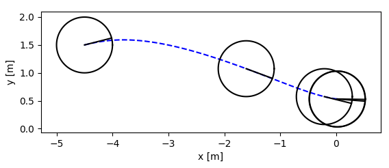
-- time history
-
-![Figure_1.png](https://qiita-image-store.s3.amazonaws.com/0/261584/e67794f3-e8ef-5162-ea84-eb6adefd4241.png)
-![Figure_2.png](https://qiita-image-store.s3.amazonaws.com/0/261584/d74fa06d-2eae-5aea-4a33-6c63e284341e.png)
-
-# Usage
-
-- for example
-
-```
-$ python main_example.py
-```
-
-- for two wheeled
-
-```
-$ python main_two_wheeled.py
-```
-
-# Requirement
-
-- python3.5 or more
-- numpy
-- matplotlib
-
-# Reference
-I`m sorry that main references are written in Japanese
-
-- main (commentary article) (Japanse)　https://qiita.com/MENDY/items/4108190a579395053924
-
-- Ohtsuka, T., & Fujii, H. A. (1997). Real-time Optimization Algorithm for Nonlinear Receding-horizon Control. Automatica, 33(6), 1147–1154. https://doi.org/10.1016/S0005-1098(97)00005-8
-
-- 非線形最適制御入門（コロナ社）
-
-- 実時間最適化による制御の実応用（コロナ社）

nmpc/cgmres/main_example.py

@@ -1,645 +0,0 @@
-import numpy as np
-import matplotlib.pyplot as plt
-import math
-
-class SampleSystem():
-    """SampleSystem, this is the simulator
-    Attributes
-    -----------
-    x_1 : float
-        system state 1
-    x_2 : float
-        system state 2
-    history_x_1 : list
-        time history of system state 1 (x_1)
-    history_x_2 : list
-        time history of system state 2 (x_2)
-    """
-    def __init__(self, init_x_1=0., init_x_2=0.):
-        """
-        Palameters
-        -----------
-        init_x_1 : float, optional
-            initial value of x_1, default is 0.
-        init_x_2 : float, optional
-            initial value of x_2, default is 0.
-        """
-        self.x_1 = init_x_1
-        self.x_2 = init_x_2
-        self.history_x_1 = [init_x_1]
-        self.history_x_2 = [init_x_2]
-
-    def update_state(self, u, dt=0.01):
-        """
-        Palameters
-        ------------
-        u : float
-            input of system in some cases this means the reference
-        dt : float in seconds, optional
-            sampling time of simulation, default is 0.01 [s]
-        """
-        # for theta 1, theta 1 dot, theta 2, theta 2 dot
-        k0 = [0.0 for _ in range(2)]
-        k1 = [0.0 for _ in range(2)]
-        k2 = [0.0 for _ in range(2)]
-        k3 = [0.0 for _ in range(2)]
-
-        functions = [self._func_x_1, self._func_x_2]
-
-        # solve Runge-Kutta
-        for i, func in enumerate(functions):
-            k0[i] = dt * func(self.x_1, self.x_2, u)
-        
-        for i, func in enumerate(functions):
-            k1[i] = dt * func(self.x_1 + k0[0]/2., self.x_2 + k0[1]/2., u)
-        
-        for i, func in enumerate(functions):
-            k2[i] = dt * func(self.x_1 + k1[0]/2., self.x_2 + k1[1]/2., u)
-        
-        for i, func in enumerate(functions):
-            k3[i] =  dt * func(self.x_1 + k2[0], self.x_2 + k2[1], u)
-        
-        self.x_1 += (k0[0] + 2. * k1[0] + 2. * k2[0] + k3[0]) / 6.
-        self.x_2 += (k0[1] + 2. * k1[1] + 2. * k2[1] + k3[1]) / 6.
-    
-        # save
-        self.history_x_1.append(self.x_1)
-        self.history_x_2.append(self.x_2)      
-
-    def _func_x_1(self, y_1, y_2, u):
-        """
-        Parameters
-        ------------
-        y_1 : float
-        y_2 : float
-        u : float
-            system input
-        """
-        y_dot = y_2
-        return y_dot
-    
-    def _func_x_2(self, y_1, y_2, u):
-        """
-        Parameters
-        ------------
-        y_1 : float
-        y_2 : float
-        u : float
-            system input
-        """
-        y_dot = (1. - y_1**2 - y_2**2) * y_2 - y_1 + u
-        return y_dot
-
-
-class NMPCSimulatorSystem():
-    """SimulatorSystem for nmpc, this is the simulator of nmpc
-    the reason why I seperate the real simulator and nmpc's simulator is sometimes the modeling error, disturbance can include in real simulator
-    Attributes
-    -----------
-    None
-
-    """
-    def __init__(self):
-        """
-        Parameters
-        -----------
-        None
-        """
-        pass
-
-    def calc_predict_and_adjoint_state(self, x_1, x_2, us, N, dt):
-        """main
-        Parameters
-        ------------
-        x_1 : float
-            current state
-        x_2 : float
-            current state
-        us : list of float
-            estimated optimal input Us for N steps
-        N : int
-            predict step
-        dt : float
-            sampling time
-
-        Returns
-        --------
-        x_1s : list of float
-            predicted x_1s for N steps
-        x_2s : list of float
-            predicted x_2s for N steps
-        lam_1s : list of float
-            adjoint state of x_1s, lam_1s for N steps
-        lam_2s : list of float
-            adjoint state of x_2s, lam_2s for N steps
-        """
-
-        x_1s, x_2s = self._calc_predict_states(x_1, x_2, us, N, dt) # by usin state equation
-        lam_1s, lam_2s = self._calc_adjoint_states(x_1s, x_2s, us, N, dt) # by using adjoint equation
-
-        return x_1s, x_2s, lam_1s, lam_2s
-
-    def _calc_predict_states(self, x_1, x_2, us, N, dt):
-        """ 
-        Parameters
-        ------------
-        x_1 : float
-            current state
-        x_2 : float
-            current state
-        us : list of float
-            estimated optimal input Us for N steps
-        N : int
-            predict step
-        dt : float
-            sampling time
-            
-        Returns
-        --------
-        x_1s : list of float
-            predicted x_1s for N steps
-        x_2s : list of float
-            predicted x_2s for N steps
-        """
-        # initial state
-        x_1s = [x_1]
-        x_2s = [x_2]
-
-        for i in range(N):
-            temp_x_1, temp_x_2 = self._predict_state_with_oylar(x_1s[i], x_2s[i], us[i], dt)
-            x_1s.append(temp_x_1)
-            x_2s.append(temp_x_2)
-
-        return x_1s, x_2s
-
-    def _calc_adjoint_states(self, x_1s, x_2s, us, N, dt):
-        """
-        Parameters
-        ------------
-        x_1s : list of float
-            predicted x_1s for N steps
-        x_2s : list of float
-            predicted x_2s for N steps
-        us : list of float
-            estimated optimal input Us for N steps
-        N : int
-            predict step
-        dt : float
-            sampling time
-            
-        Returns
-        --------
-        lam_1s : list of float
-            adjoint state of x_1s, lam_1s for N steps
-        lam_2s : list of float
-            adjoint state of x_2s, lam_2s for N steps
-        """
-        # final state
-        # final_state_func
-        lam_1s = [x_1s[-1]]
-        lam_2s = [x_2s[-1]]
-
-        for i in range(N-1, 0, -1): 
-            temp_lam_1, temp_lam_2 = self._adjoint_state_with_oylar(x_1s[i], x_2s[i], lam_1s[0] ,lam_2s[0], us[i], dt)
-            lam_1s.insert(0, temp_lam_1)
-            lam_2s.insert(0, temp_lam_2)
-
-        return lam_1s, lam_2s
-
-    def final_state_func(self):
-        """this func usually need
-        """
-        pass
-
-    def _predict_state_with_oylar(self, x_1, x_2, u, dt):
-        """in this case this function is the same as simulator
-        Parameters
-        ------------
-        x_1 : float
-            system state
-        x_2 : float
-            system state
-        u : float
-            system input
-        dt : float in seconds
-            sampling time
-        Returns
-        --------
-        next_x_1 : float
-            next state, x_1 calculated by using state equation
-        next_x_2 : float
-            next state, x_2 calculated by using state equation
-        """
-        k0 = [0. for _ in range(2)]
-
-        functions = [self.func_x_1, self.func_x_2]
-
-        for i, func in enumerate(functions):
-            k0[i] = dt * func(x_1, x_2, u)
-                
-        next_x_1 = x_1 + k0[0]
-        next_x_2 = x_2 + k0[1]
-
-        return next_x_1, next_x_2
-
-    def func_x_1(self, y_1, y_2, u):
-        """calculating \dot{x_1}
-        Parameters
-        ------------
-        y_1 : float
-            means x_1
-        y_2 : float
-            means x_2
-        u : float
-            means system input
-        Returns
-        ---------
-        y_dot : float
-            means \dot{x_1}
-        """
-        y_dot = y_2
-        return y_dot
-    
-    def func_x_2(self, y_1, y_2, u):
-        """calculating \dot{x_2}
-        Parameters
-        ------------
-        y_1 : float
-            means x_1
-        y_2 : float
-            means x_2
-        u : float
-            means system input
-        Returns
-        ---------
-        y_dot : float
-            means \dot{x_2}
-        """
-        y_dot = (1. - y_1**2 - y_2**2) * y_2 - y_1 + u
-        return y_dot
-
-    def _adjoint_state_with_oylar(self, x_1, x_2, lam_1, lam_2, u, dt):
-        """
-        Parameters
-        ------------
-        x_1 : float
-            system state
-        x_2 : float
-            system state
-        lam_1 : float
-            adjoint state
-        lam_2 : float
-            adjoint state
-        u : float
-            system input
-        dt : float in seconds
-            sampling time
-        Returns
-        --------
-        pre_lam_1 : float
-            pre, 1 step before lam_1 calculated by using adjoint equation
-        pre_lam_2 : float
-            pre, 1 step before lam_2 calculated by using adjoint equation
-        """
-        k0 = [0. for _ in range(2)]
-
-        functions = [self._func_lam_1, self._func_lam_2]
-
-        for i, func in enumerate(functions):
-            k0[i] = dt * func(x_1, x_2, lam_1, lam_2, u)
-                
-        pre_lam_1 = lam_1 + k0[0]
-        pre_lam_2 = lam_2 + k0[1]
-
-        return pre_lam_1, pre_lam_2
-
-    def _func_lam_1(self, y_1, y_2, y_3, y_4, u):
-        """calculating -\dot{lam_1}
-        Parameters
-        ------------
-        y_1 : float
-            means x_1
-        y_2 : float
-            means x_2
-        y_3 : float
-            means lam_1
-        y_4 : float
-            means lam_2
-        u : float
-            means system input
-        Returns
-        ---------
-        y_dot : float
-            means -\dot{lam_1}
-        """
-        y_dot = y_1 - (2. * y_1 * y_2 + 1.) * y_4
-        return y_dot
-
-    def _func_lam_2(self, y_1, y_2, y_3, y_4, u):
-        """calculating -\dot{lam_2}
-        Parameters
-        ------------
-        y_1 : float
-            means x_1
-        y_2 : float
-            means x_2
-        y_3 : float
-            means lam_1
-        y_4 : float
-            means lam_2
-        u : float
-            means system input
-        Returns
-        ---------
-        y_dot : float
-            means -\dot{lam_2}
-        """
-        y_dot = y_2 + y_3 + (-3. * (y_2**2) - y_1**2 + 1. ) * y_4
-        return y_dot
-
-class NMPCController_with_CGMRES():
-    """
-    Attributes
-    ------------
-    zeta : float
-        gain of optimal answer stability
-    ht : float
-        update value of NMPC this should be decided by zeta
-    tf : float
-        predict time
-    alpha : float
-        gain of predict time
-    N : int
-        predicte step, discritize value
-    threshold : float
-        cgmres's threshold value
-    input_num : int
-        system input length, this should include dummy u and constraint variables
-    max_iteration : int
-        decide by the solved matrix size
-    simulator : NMPCSimulatorSystem class
-    us : list of float
-        estimated optimal system input
-    dummy_us : list of float
-        estimated dummy input
-    raws : list of float
-        estimated constraint variable
-    history_u : list of float
-        time history of actual system input
-    history_dummy_u : list of float
-        time history of actual dummy u
-    history_raw : list of float
-        time history of actual raw
-    history_f : list of float
-        time history of error of optimal
-    """
-    def __init__(self):
-        """
-        Parameters
-        -----------
-        None
-        """
-        # parameters
-        self.zeta = 100. # 安定化ゲイン
-        self.ht = 0.01 # 差分近似の幅
-        self.tf = 1. # 最終時間
-        self.alpha = 0.5 # 時間の上昇ゲイン
-        self.N = 10 # 分割数
-        self.threshold = 0.001 # break値
-
-        self.input_num = 3 # dummy, 制約条件に対するuにも合わせた入力の数
-        self.max_iteration = self.input_num * self.N
-
-        # simulator
-        self.simulator = NMPCSimulatorSystem()
-
-        # initial
-        self.us = np.zeros(self.N)
-        self.dummy_us = np.ones(self.N) * 0.49
-        self.raws = np.ones(self.N) * 0.011
-
-        # for fig
-        self.history_u = []
-        self.history_dummy_u = []
-        self.history_raw = []
-        self.history_f = []
-
-    def calc_input(self, x_1, x_2, time):
-        """
-        Parameters
-        ------------
-        x_1 : float
-            current state
-        x_2 : float
-            current state
-        time : float in seconds
-            now time
-        Returns
-        --------
-        us : list of float
-            estimated optimal system input
-        """
-        # calculating sampling time
-        dt = self.tf * (1. - np.exp(-self.alpha * time)) / float(self.N)
-
-        # x_dot
-        x_1_dot = self.simulator.func_x_1(x_1, x_2, self.us[0])
-        x_2_dot = self.simulator.func_x_2(x_1, x_2, self.us[0])
-
-        dx_1 = x_1_dot * self.ht
-        dx_2 = x_2_dot * self.ht
-
-        x_1s, x_2s, lam_1s, lam_2s = self.simulator.calc_predict_and_adjoint_state(x_1 + dx_1, x_2 + dx_2, self.us, self.N, dt)
-        
-        # Fxt
-        Fxt = self._calc_f(x_1s, x_2s, lam_1s, lam_2s, self.us, self.dummy_us,
-                            self.raws, self.N, dt)
-
-        # F
-        x_1s, x_2s, lam_1s, lam_2s = self.simulator.calc_predict_and_adjoint_state(x_1, x_2, self.us, self.N, dt)
-
-        F = self._calc_f(x_1s, x_2s, lam_1s, lam_2s, self.us, self.dummy_us,
-                            self.raws, self.N, dt)
-
-        right = -self.zeta * F - ((Fxt - F) / self.ht)
-
-        du = self.us * self.ht
-        ddummy_u = self.dummy_us * self.ht
-        draw = self.raws * self.ht
-
-        x_1s, x_2s, lam_1s, lam_2s = self.simulator.calc_predict_and_adjoint_state(x_1 + dx_1, x_2 + dx_2, self.us + du, self.N, dt)
-
-        Fuxt = self._calc_f(x_1s, x_2s, lam_1s, lam_2s, self.us + du, self.dummy_us + ddummy_u,
-                           self.raws + draw, self.N, dt)
-
-        left = ((Fuxt - Fxt) / self.ht)
-
-        # calculationg cgmres
-        r0 = right - left
-        r0_norm = np.linalg.norm(r0)
-        
-        vs = np.zeros((self.max_iteration, self.max_iteration + 1)) # 数×iterarion回数
-        
-        vs[:, 0] = r0 / r0_norm # 最初の基底を算出
-
-        hs = np.zeros((self.max_iteration + 1, self.max_iteration + 1))
-
-        e = np.zeros((self.max_iteration + 1, 1)) # in this case the state is 3(u and dummy_u)
-        e[0] = 1.
-
-        for i in range(self.max_iteration):
-            du = vs[::3, i] * self.ht
-            ddummy_u = vs[1::3, i] * self.ht
-            draw = vs[2::3, i] * self.ht
-
-            x_1s, x_2s, lam_1s, lam_2s = self.simulator.calc_predict_and_adjoint_state(x_1 + dx_1, x_2 + dx_2, self.us + du, self.N, dt)
-
-            Fuxt = self._calc_f(x_1s, x_2s, lam_1s, lam_2s, self.us + du, self.dummy_us + ddummy_u,
-                           self.raws + draw, self.N, dt)
-
-            Av = (( Fuxt - Fxt) / self.ht)
-
-            sum_Av = np.zeros(self.max_iteration)
-
-            for j in range(i + 1): # グラムシュミットの直交化法です、和を取って差分を取って算出します
-                hs[j, i] = np.dot(Av, vs[:, j])
-                sum_Av = sum_Av + hs[j, i] * vs[:, j]
-
-            v_est = Av - sum_Av
-
-            hs[i+1, i] = np.linalg.norm(v_est)
-
-            vs[:, i+1] = v_est / hs[i+1, i]
-
-            inv_hs = np.linalg.pinv(hs[:i+1, :i]) # この辺は教科書（実時間の方）にのっています
-            ys = np.dot(inv_hs, r0_norm * e[:i+1])
-
-            judge_value = r0_norm * e[:i+1] - np.dot(hs[:i+1, :i], ys[:i])
-
-            if np.linalg.norm(judge_value) < self.threshold or i == self.max_iteration-1:
-                update_value = np.dot(vs[:, :i-1], ys_pre[:i-1]).flatten()
-                du_new = du + update_value[::3]
-                ddummy_u_new = ddummy_u + update_value[1::3]
-                draw_new = draw + update_value[2::3]
-                break
-
-            ys_pre = ys
-        
-        # update
-        self.us += du_new * self.ht
-        self.dummy_us += ddummy_u_new * self.ht
-        self.raws += draw_new * self.ht
-
-        x_1s, x_2s, lam_1s, lam_2s = self.simulator.calc_predict_and_adjoint_state(x_1, x_2, self.us, self.N, dt)
-
-        F = self._calc_f(x_1s, x_2s, lam_1s, lam_2s, self.us, self.dummy_us,
-                            self.raws, self.N, dt)
-
-        print("check F = {0}".format(np.linalg.norm(F)))
-
-        # for save
-        self.history_f.append(np.linalg.norm(F))
-        self.history_u.append(self.us[0])
-        self.history_dummy_u.append(self.dummy_us[0])
-        self.history_raw.append(self.raws[0])
-
-        return self.us
-
-    def _calc_f(self, x_1s, x_2s, lam_1s, lam_2s, us, dummy_us, raws, N, dt):
-        """
-        Parameters
-        ------------
-        x_1s : list of float
-            predicted x_1s for N steps
-        x_2s : list of float
-            predicted x_2s for N steps
-        lam_1s : list of float
-            adjoint state of x_1s, lam_1s for N steps
-        lam_2s : list of float
-            adjoint state of x_2s, lam_2s for N steps
-        us : list of float
-            estimated optimal system input
-        dummy_us : list of float
-            estimated dummy input
-        raws : list of float
-            estimated constraint variable
-        N : int
-            predict time step
-        dt : float
-            sampling time of system
-        """
-        F = []
-
-        for i in range(N):
-            F.append(us[i] + lam_2s[i] + 2. * raws[i] * us[i])
-            F.append(-0.01 + 2. * raws[i] * dummy_us[i])
-            F.append(us[i]**2 + dummy_us[i]**2 - 0.5**2)
-        
-        return np.array(F)
-
-def main():
-    # simulation time
-    dt = 0.01
-    iteration_time = 20.
-    iteration_num = int(iteration_time/dt)
-
-    # plant
-    plant_system = SampleSystem(init_x_1=2., init_x_2=0.)
-
-    # controller
-    controller = NMPCController_with_CGMRES()
-
-    # for i in range(iteration_num)
-    for i in range(1, iteration_num):
-        time = float(i) * dt
-        x_1 = plant_system.x_1
-        x_2 = plant_system.x_2
-        # make input
-        us = controller.calc_input(x_1, x_2, time)
-        # update state
-        plant_system.update_state(us[0])
-    
-    # figure
-    fig = plt.figure()
-
-    x_1_fig = fig.add_subplot(321)
-    x_2_fig = fig.add_subplot(322)
-    u_fig = fig.add_subplot(323)
-    dummy_fig = fig.add_subplot(324)
-    raw_fig = fig.add_subplot(325)
-    f_fig = fig.add_subplot(326)
-
-    x_1_fig.plot(np.arange(iteration_num)*dt, plant_system.history_x_1)
-    x_1_fig.set_xlabel("time [s]")
-    x_1_fig.set_ylabel("x_1")
-    
-    x_2_fig.plot(np.arange(iteration_num)*dt, plant_system.history_x_2)
-    x_2_fig.set_xlabel("time [s]")
-    x_2_fig.set_ylabel("x_2")
-    
-    u_fig.plot(np.arange(iteration_num - 1)*dt, controller.history_u)
-    u_fig.set_xlabel("time [s]")
-    u_fig.set_ylabel("u")
-
-    dummy_fig.plot(np.arange(iteration_num - 1)*dt, controller.history_dummy_u)
-    dummy_fig.set_xlabel("time [s]")
-    dummy_fig.set_ylabel("dummy u")
-
-    raw_fig.plot(np.arange(iteration_num - 1)*dt, controller.history_raw)
-    raw_fig.set_xlabel("time [s]")
-    raw_fig.set_ylabel("raw")
-
-    f_fig.plot(np.arange(iteration_num - 1)*dt, controller.history_f)
-    f_fig.set_xlabel("time [s]")
-    f_fig.set_ylabel("optimal error")
-
-    fig.tight_layout()
-
-    plt.show()
-
-
-if __name__ == "__main__":
-    main()
-
-
-    

nmpc/cgmres/main_two_wheeled.py

@@ -1,893 +0,0 @@
-import numpy as np
-import matplotlib.pyplot as plt
-import math
-
-class TwoWheeledSystem():
-    """SampleSystem, this is the simulator
-    Attributes
-    -----------
-    x_1 : float
-        system state 1
-    x_2 : float
-        system state 2
-    history_x_1 : list
-        time history of system state 1 (x_1)
-    history_x_2 : list
-        time history of system state 2 (x_2)
-    """
-    def __init__(self, init_x_1=0., init_x_2=0., init_x_3=0.):
-        """
-        Palameters
-        -----------
-        init_x_1 : float, optional
-            initial value of x_1, default is 0.
-        init_x_2 : float, optional
-            initial value of x_2, default is 0.
-        init_x_3 : float, optional
-            initial value of x_3, default is 0.
-        """
-        self.x_1 = init_x_1
-        self.x_2 = init_x_2
-        self.x_3 = init_x_3
-        self.history_x_1 = [init_x_1]
-        self.history_x_2 = [init_x_2]
-        self.history_x_3 = [init_x_3]
-
-    def update_state(self, u_1, u_2, dt=0.01):
-        """
-        Palameters
-        ------------
-        u_1 : float
-            input of system in some cases this means the reference, u_velocity
-        u_2 : float
-            input of system in some cases this means the reference, u_omega
-        dt : float in seconds, optional
-            sampling time of simulation, default is 0.01 [s]
-        """
-        # for theta 1, theta 1 dot, theta 2, theta 2 dot
-        k0 = [0.0 for _ in range(3)]
-        k1 = [0.0 for _ in range(3)]
-        k2 = [0.0 for _ in range(3)]
-        k3 = [0.0 for _ in range(3)]
-
-        functions = [self._func_x_1, self._func_x_2, self._func_x_3]
-
-        # solve Runge-Kutta
-        for i, func in enumerate(functions):
-            k0[i] = dt * func(self.x_1, self.x_2, self.x_3, u_1, u_2)
-        
-        for i, func in enumerate(functions):
-            k1[i] = dt * func(self.x_1 + k0[0]/2., self.x_2 + k0[1]/2., self.x_3 + k0[2]/2., u_1, u_2)
-        
-        for i, func in enumerate(functions):
-            k2[i] = dt * func(self.x_1 + k1[0]/2., self.x_2 + k1[1]/2., self.x_3 + k1[2]/2., u_1, u_2)
-        
-        for i, func in enumerate(functions):
-            k3[i] =  dt * func(self.x_1 + k2[0], self.x_2 + k2[1], self.x_3 + k2[2], u_1, u_2)
-        
-        self.x_1 += (k0[0] + 2. * k1[0] + 2. * k2[0] + k3[0]) / 6.
-        self.x_2 += (k0[1] + 2. * k1[1] + 2. * k2[1] + k3[1]) / 6.
-        self.x_3 += (k0[2] + 2. * k1[2] + 2. * k2[2] + k3[2]) / 6.
-    
-        # save
-        self.history_x_1.append(self.x_1)
-        self.history_x_2.append(self.x_2)
-        self.history_x_3.append(self.x_3)      
-
-    def _func_x_1(self, y_1, y_2, y_3, u_1, u_2):
-        """
-        Parameters
-        ------------
-        y_1 : float
-        y_2 : float
-        y_3 : float
-        u_1 : float
-            system input
-        u_2 : float
-            system input
-        """
-        y_dot = math.cos(y_3) * u_1
-        return y_dot
-    
-    def _func_x_2(self, y_1, y_2, y_3, u_1, u_2):
-        """
-        Parameters
-        ------------
-        y_1 : float
-        y_2 : float
-        y_3 : float
-        u_1 : float
-            system input
-        u_2 : float
-            system input
-        """
-        y_dot = math.sin(y_3) * u_1
-        return y_dot
-    
-    def _func_x_3(self, y_1, y_2, y_3, u_1, u_2):
-        """
-        Parameters
-        ------------
-        y_1 : float
-        y_2 : float
-        y_3 : float
-        u_1 : float
-            system input
-        u_2 : float
-            system input
-        """
-        y_dot = u_2
-        return y_dot
-
-class NMPCSimulatorSystem():
-    """SimulatorSystem for nmpc, this is the simulator of nmpc
-    the reason why I seperate the real simulator and nmpc's simulator is sometimes the modeling error, disturbance can include in real simulator
-    Attributes
-    -----------
-    None
-
-    """
-    def __init__(self):
-        """
-        Parameters
-        -----------
-        None
-        """
-        pass
-
-    def calc_predict_and_adjoint_state(self, x_1, x_2, x_3, u_1s, u_2s, N, dt):
-        """main
-        Parameters
-        ------------
-        x_1 : float
-            current state
-        x_2 : float
-            current state
-        x_3 : float
-            current state
-        u_1s : list of float
-            estimated optimal input Us for N steps
-        u_2s : list of float
-            estimated optimal input Us for N steps
-        N : int
-            predict step
-        dt : float
-            sampling time
-
-        Returns
-        --------
-        x_1s : list of float
-            predicted x_1s for N steps
-        x_2s : list of float
-            predicted x_2s for N steps
-        x_3s : list of float
-            predicted x_3s for N steps
-        lam_1s : list of float
-            adjoint state of x_1s, lam_1s for N steps
-        lam_2s : list of float
-            adjoint state of x_2s, lam_2s for N steps
-        lam_3s : list of float
-            adjoint state of x_3s, lam_3s for N steps
-        """
-        x_1s, x_2s, x_3s = self._calc_predict_states(x_1, x_2, x_3, u_1s, u_2s, N, dt) # by usin state equation
-        lam_1s, lam_2s, lam_3s = self._calc_adjoint_states(x_1s, x_2s, x_3s, u_1s, u_2s, N, dt) # by using adjoint equation
-
-        return x_1s, x_2s, x_3s, lam_1s, lam_2s, lam_3s
-
-    def _calc_predict_states(self, x_1, x_2, x_3, u_1s, u_2s, N, dt):
-        """ 
-        Parameters
-        ------------
-        x_1 : float
-            current state
-        x_2 : float
-            current state
-        x_3 : float
-            current state
-        u_1s : list of float
-            estimated optimal input Us for N steps
-        u_2s : list of float
-            estimated optimal input Us for N steps
-        N : int
-            predict step
-        dt : float
-            sampling time
-            
-        Returns
-        --------
-        x_1s : list of float
-            predicted x_1s for N steps
-        x_2s : list of float
-            predicted x_2s for N steps
-        x_3s : list of float
-            predicted x_3s for N steps
-        """
-        # initial state
-        x_1s = [x_1]
-        x_2s = [x_2]
-        x_3s = [x_3]
-
-        for i in range(N):
-            temp_x_1, temp_x_2, temp_x_3 = self._predict_state_with_oylar(x_1s[i], x_2s[i], x_3s[i], u_1s[i], u_2s[i], dt)
-            x_1s.append(temp_x_1)
-            x_2s.append(temp_x_2)
-            x_3s.append(temp_x_3)
-
-        return x_1s, x_2s, x_3s
-
-    def _calc_adjoint_states(self, x_1s, x_2s, x_3s, u_1s, u_2s, N, dt):
-        """
-        Parameters
-        ------------
-        x_1s : list of float
-            predicted x_1s for N steps
-        x_2s : list of float
-            predicted x_2s for N steps
-        x_3s : list of float
-            predicted x_3s for N steps
-        u_1s : list of float
-            estimated optimal input Us for N steps
-        u_2s : list of float
-            estimated optimal input Us for N steps
-        N : int
-            predict step
-        dt : float
-            sampling time
-            
-        Returns
-        --------
-        lam_1s : list of float
-            adjoint state of x_1s, lam_1s for N steps
-        lam_2s : list of float
-            adjoint state of x_2s, lam_2s for N steps
-        lam_3s : list of float
-            adjoint state of x_2s, lam_2s for N steps
-        """
-        # final state
-        # final_state_func
-        lam_1s = [x_1s[-1]]
-        lam_2s = [x_2s[-1]]
-        lam_3s = [x_3s[-1]]
-
-        for i in range(N-1, 0, -1): 
-            temp_lam_1, temp_lam_2, temp_lam_3 = self._adjoint_state_with_oylar(x_1s[i], x_2s[i], x_3s[i], lam_1s[0] ,lam_2s[0], lam_3s[0], u_1s[i], u_2s[i], dt)
-            lam_1s.insert(0, temp_lam_1)
-            lam_2s.insert(0, temp_lam_2)
-            lam_3s.insert(0, temp_lam_3)
-
-        return lam_1s, lam_2s, lam_3s
-
-    def final_state_func(self):
-        """this func usually need
-        """
-        pass
-
-    def _predict_state_with_oylar(self, x_1, x_2, x_3, u_1, u_2, dt):
-        """in this case this function is the same as simulator
-        Parameters
-        ------------
-        x_1 : float
-            system state
-        x_2 : float
-            system state
-        x_3 : float
-            system state
-        u_1 : float
-            system input
-        u_2 : float
-            system input
-        dt : float in seconds
-            sampling time
-        Returns
-        --------
-        next_x_1 : float
-            next state, x_1 calculated by using state equation
-        next_x_2 : float
-            next state, x_2 calculated by using state equation
-        next_x_3 : float
-            next state, x_3 calculated by using state equation
-        """
-        k0 = [0. for _ in range(3)]
-
-        functions = [self.func_x_1, self.func_x_2, self.func_x_3]
-
-        for i, func in enumerate(functions):
-            k0[i] = dt * func(x_1, x_2, x_3, u_1, u_2)
-                
-        next_x_1 = x_1 + k0[0]
-        next_x_2 = x_2 + k0[1]
-        next_x_3 = x_3 + k0[2]
-
-        return next_x_1, next_x_2, next_x_3
-
-    def func_x_1(self, y_1, y_2, y_3, u_1, u_2):
-        """
-        Parameters
-        ------------
-        y_1 : float
-        y_2 : float
-        y_3 : float
-        u_1 : float
-            system input
-        u_2 : float
-            system input
-        """
-        y_dot = math.cos(y_3) * u_1
-        return y_dot
-    
-    def func_x_2(self, y_1, y_2, y_3, u_1, u_2):
-        """
-        Parameters
-        ------------
-        y_1 : float
-        y_2 : float
-        y_3 : float
-        u_1 : float
-            system input
-        u_2 : float
-            system input
-        """
-        y_dot = math.sin(y_3) * u_1
-        return y_dot
-    
-    def func_x_3(self, y_1, y_2, y_3, u_1, u_2):
-        """
-        Parameters
-        ------------
-        y_1 : float
-        y_2 : float
-        y_3 : float
-        u_1 : float
-            system input
-        u_2 : float
-            system input
-        """
-        y_dot = u_2
-        return y_dot
-
-    def _adjoint_state_with_oylar(self, x_1, x_2, x_3, lam_1, lam_2, lam_3, u_1, u_2, dt):
-        """
-        Parameters
-        ------------
-        x_1 : float
-            system state
-        x_2 : float
-            system state
-        x_3 : float
-            system state
-        lam_1 : float
-            adjoint state
-        lam_2 : float
-            adjoint state
-        lam_3 : float
-            adjoint state
-        u_1 : float
-            system input
-        u_2 : float
-            system input
-        dt : float in seconds
-            sampling time
-        Returns
-        --------
-        pre_lam_1 : float
-            pre, 1 step before lam_1 calculated by using adjoint equation
-        pre_lam_2 : float
-            pre, 1 step before lam_2 calculated by using adjoint equation
-        pre_lam_3 : float
-            pre, 1 step before lam_3 calculated by using adjoint equation
-        """
-        k0 = [0. for _ in range(3)]
-
-        functions = [self._func_lam_1, self._func_lam_2, self._func_lam_3]
-
-        for i, func in enumerate(functions):
-            k0[i] = dt * func(x_1, x_2, x_3, lam_1, lam_2, lam_3, u_1, u_2)
-                
-        pre_lam_1 = lam_1 + k0[0]
-        pre_lam_2 = lam_2 + k0[1]
-        pre_lam_3 = lam_3 + k0[2]
-
-        return pre_lam_1, pre_lam_2, pre_lam_3
-
-    def _func_lam_1(self, y_1, y_2, y_3, y_4, y_5, y_6, u_1, u_2):
-        """calculating -\dot{lam_1}
-        Parameters
-        ------------
-        y_1 : float
-            means x_1
-        y_2 : float
-            means x_2
-        y_3 : float
-            means x_3
-        y_4 : float
-            means lam_1
-        y_5 : float
-            means lam_2
-        y_6 : float
-            means lam_3
-        u_1 : float
-            means system input
-        u_2 : float
-            means system input
-        Returns
-        ---------
-        y_dot : float
-            means -\dot{lam_1}
-        """
-        y_dot = 0.
-        return y_dot
-
-    def _func_lam_2(self, y_1, y_2, y_3, y_4, y_5, y_6, u_1, u_2):
-        """calculating -\dot{lam_2}
-        Parameters
-        ------------
-        y_1 : float
-            means x_1
-        y_2 : float
-            means x_2
-        y_3 : float
-            means x_3
-        y_4 : float
-            means lam_1
-        y_5 : float
-            means lam_2
-        y_6 : float
-            means lam_3
-        u_1 : float
-            means system input
-        u_2 : float
-            means system input
-        Returns
-        ---------
-        y_dot : float
-            means -\dot{lam_2}
-        """
-        y_dot = 0.
-        return y_dot
-
-    def _func_lam_3(self, y_1, y_2, y_3, y_4, y_5, y_6, u_1, u_2):
-        """calculating -\dot{lam_3}
-        Parameters
-        ------------
-        y_1 : float
-            means x_1
-        y_2 : float
-            means x_2
-        y_3 : float
-            means x_3
-        y_4 : float
-            means lam_1
-        y_5 : float
-            means lam_2
-        y_6 : float
-            means lam_3
-        u_1 : float
-            means system input
-        u_2 : float
-            means system input
-        Returns
-        ---------
-        y_dot : float
-            means -\dot{lam_3}
-        """
-        y_dot = - y_4 * math.sin(y_3) * u_1 + y_5 * math.cos(y_3) * u_1 
-        return y_dot
-
-class NMPCController_with_CGMRES():
-    """
-    Attributes
-    ------------
-    zeta : float
-        gain of optimal answer stability
-    ht : float
-        update value of NMPC this should be decided by zeta
-    tf : float
-        predict time
-    alpha : float
-        gain of predict time
-    N : int
-        predicte step, discritize value
-    threshold : float
-        cgmres's threshold value
-    input_num : int
-        system input length, this should include dummy u and constraint variables
-    max_iteration : int
-        decide by the solved matrix size
-    simulator : NMPCSimulatorSystem class
-    u_1s : list of float
-        estimated optimal system input
-    u_2s : list of float
-        estimated optimal system input
-    dummy_u_1s : list of float
-        estimated dummy input
-    dummy_u_2s : list of float
-        estimated dummy input
-    raw_1s : list of float
-        estimated constraint variable
-    raw_2s : list of float
-        estimated constraint variable
-    history_u_1 : list of float
-        time history of actual system input
-    history_u_2 : list of float
-        time history of actual system input
-    history_dummy_u_1 : list of float
-        time history of actual dummy u_1
-    history_dummy_u_2 : list of float
-        time history of actual dummy u_2
-    history_raw_1 : list of float
-        time history of actual raw_1
-    history_raw_2 : list of float
-        time history of actual raw_2
-    history_f : list of float
-        time history of error of optimal
-    """
-    def __init__(self):
-        """
-        Parameters
-        -----------
-        None
-        """
-        # parameters
-        self.zeta = 100. # 安定化ゲイン
-        self.ht = 0.01 # 差分近似の幅
-        self.tf = 1. # 最終時間
-        self.alpha = 0.5 # 時間の上昇ゲイン
-        self.N = 10 # 分割数
-        self.threshold = 0.001 # break値
-
-        self.input_num = 6 # dummy, 制約条件に対するuにも合わせた入力の数
-        self.max_iteration = self.input_num * self.N
-
-        # simulator
-        self.simulator = NMPCSimulatorSystem()
-
-        # initial
-        self.u_1s = np.ones(self.N) * 1.
-        self.u_2s = np.ones(self.N) * 0.1
-        self.dummy_u_1s = np.ones(self.N) * 0.1
-        self.dummy_u_2s = np.ones(self.N) * 2.5
-        self.raw_1s = np.ones(self.N) * 0.8
-        self.raw_2s = np.ones(self.N) * 0.8
-
-        # for fig
-        self.history_u_1 = []
-        self.history_u_2 = []
-        self.history_dummy_u_1 = []
-        self.history_dummy_u_2 = []
-        self.history_raw_1 = []
-        self.history_raw_2 = []
-        self.history_f = []
-
-    def calc_input(self, x_1, x_2, x_3, time):
-        """
-        Parameters
-        ------------
-        x_1 : float
-            current state
-        x_2 : float
-            current state
-        x_3 : float
-            current state
-        time : float in seconds
-            now time
-        Returns
-        --------
-        u_1s : list of float
-            estimated optimal system input
-        u_2s : list of float
-            estimated optimal system input
-        """
-        # calculating sampling time
-        dt = self.tf * (1. - np.exp(-self.alpha * time)) / float(self.N)
-
-        # x_dot
-        x_1_dot = self.simulator.func_x_1(x_1, x_2,  x_3, self.u_1s[0], self.u_2s[0])
-        x_2_dot = self.simulator.func_x_2(x_1, x_2, x_3, self.u_1s[0], self.u_2s[0])
-        x_3_dot = self.simulator.func_x_3(x_1, x_2, x_3, self.u_1s[0], self.u_2s[0])
-
-        dx_1 = x_1_dot * self.ht
-        dx_2 = x_2_dot * self.ht
-        dx_3 = x_3_dot * self.ht
-
-        x_1s, x_2s, x_3s, lam_1s, lam_2s, lam_3s = self.simulator.calc_predict_and_adjoint_state(x_1 + dx_1, x_2 + dx_2,  x_3 + dx_3, self.u_1s, self.u_2s, self.N, dt)
-        
-        # Fxt
-        Fxt = self._calc_f(x_1s, x_2s, x_3s, lam_1s, lam_2s, lam_3s, self.u_1s, self.u_2s, self.dummy_u_1s,  self.dummy_u_2s,
-                            self.raw_1s, self.raw_2s, self.N, dt)
-
-        # F
-        x_1s, x_2s, x_3s, lam_1s, lam_2s, lam_3s = self.simulator.calc_predict_and_adjoint_state(x_1, x_2, x_3, self.u_1s, self.u_2s, self.N, dt)
-
-        F = self._calc_f(x_1s, x_2s, x_3s, lam_1s, lam_2s, lam_3s, self.u_1s, self.u_2s, self.dummy_u_1s,  self.dummy_u_2s,
-                            self.raw_1s, self.raw_2s, self.N, dt)
-
-        right = -self.zeta * F - ((Fxt - F) / self.ht)
-
-        du_1 = self.u_1s * self.ht
-        du_2 = self.u_2s * self.ht
-        ddummy_u_1 = self.dummy_u_1s * self.ht
-        ddummy_u_2 = self.dummy_u_2s * self.ht
-        draw_1 = self.raw_1s * self.ht
-        draw_2 = self.raw_2s * self.ht
-
-        x_1s, x_2s, x_3s, lam_1s, lam_2s, lam_3s = self.simulator.calc_predict_and_adjoint_state(x_1 + dx_1, x_2 + dx_2, x_3 + dx_3, self.u_1s + du_1, self.u_2s + du_2, self.N, dt)
-
-        Fuxt = self._calc_f(x_1s, x_2s, x_3s, lam_1s, lam_2s, lam_3s, self.u_1s + du_1, self.u_2s + du_2, self.dummy_u_1s + ddummy_u_1,  self.dummy_u_2s + ddummy_u_2, 
-                           self.raw_1s + draw_1, self.raw_2s + draw_2, self.N, dt)
-
-        left = ((Fuxt - Fxt) / self.ht)
-
-        # calculationg cgmres
-        r0 = right - left
-        r0_norm = np.linalg.norm(r0)
-        
-        vs = np.zeros((self.max_iteration, self.max_iteration + 1)) # 数×iterarion回数
-        
-        vs[:, 0] = r0 / r0_norm # 最初の基底を算出
-
-        hs = np.zeros((self.max_iteration + 1, self.max_iteration + 1))
-
-        e = np.zeros((self.max_iteration + 1, 1)) # in this case the state is 3(u and dummy_u)
-        e[0] = 1.
-
-        for i in range(self.max_iteration):
-            du_1 = vs[::self.input_num, i] * self.ht
-            du_2 = vs[1::self.input_num, i] * self.ht
-            ddummy_u_1 = vs[2::self.input_num, i] * self.ht
-            ddummy_u_2 = vs[3::self.input_num, i] * self.ht            
-            draw_1 = vs[4::self.input_num, i] * self.ht
-            draw_2 = vs[5::self.input_num, i] * self.ht
-
-            x_1s, x_2s, x_3s, lam_1s, lam_2s, lam_3s = self.simulator.calc_predict_and_adjoint_state(x_1 + dx_1, x_2 + dx_2, x_3 + dx_3, self.u_1s + du_1, self.u_2s + du_2, self.N, dt)
-
-            Fuxt = self._calc_f(x_1s, x_2s, x_3s, lam_1s, lam_2s, lam_3s, self.u_1s + du_1, self.u_2s + du_2, self.dummy_u_1s + ddummy_u_1,  self.dummy_u_2s + ddummy_u_2, 
-                           self.raw_1s + draw_1, self.raw_2s + draw_2, self.N, dt)
-
-            Av = (( Fuxt - Fxt) / self.ht)
-
-            sum_Av = np.zeros(self.max_iteration)
-
-            for j in range(i + 1): # グラムシュミットの直交化法です、和を取って差分を取って算出します
-                hs[j, i] = np.dot(Av, vs[:, j])
-                sum_Av = sum_Av + hs[j, i] * vs[:, j]
-
-            v_est = Av - sum_Av
-
-            hs[i+1, i] = np.linalg.norm(v_est)
-
-            vs[:, i+1] = v_est / hs[i+1, i]
-
-            inv_hs = np.linalg.pinv(hs[:i+1, :i]) # この辺は教科書（実時間の方）にのっています
-            ys = np.dot(inv_hs, r0_norm * e[:i+1])
-
-            judge_value = r0_norm * e[:i+1] - np.dot(hs[:i+1, :i], ys[:i])
-
-            if np.linalg.norm(judge_value) < self.threshold or i == self.max_iteration-1:
-                update_value = np.dot(vs[:, :i-1], ys_pre[:i-1]).flatten()
-                du_1_new = du_1 + update_value[::self.input_num]
-                du_2_new = du_2 + update_value[1::self.input_num]
-                ddummy_u_1_new = ddummy_u_1 + update_value[2::self.input_num]
-                ddummy_u_2_new = ddummy_u_2 + update_value[3::self.input_num]
-                draw_1_new = draw_1 + update_value[4::self.input_num]
-                draw_2_new = draw_2 + update_value[5::self.input_num]
-                break
-
-            ys_pre = ys
-        
-        # update
-        self.u_1s += du_1_new * self.ht
-        self.u_2s += du_2_new * self.ht
-        self.dummy_u_1s += ddummy_u_1_new * self.ht
-        self.dummy_u_2s += ddummy_u_2_new * self.ht
-        self.raw_1s += draw_1_new * self.ht
-        self.raw_2s += draw_2_new * self.ht
-
-        x_1s, x_2s, x_3s, lam_1s, lam_2s, lam_3s = self.simulator.calc_predict_and_adjoint_state(x_1, x_2, x_3, self.u_1s, self.u_2s, self.N, dt)
-
-        F = self._calc_f(x_1s, x_2s, x_3s, lam_1s, lam_2s, lam_3s, self.u_1s, self.u_2s, self.dummy_u_1s,  self.dummy_u_2s,
-                         self.raw_1s, self.raw_2s, self.N, dt)
-
-        print("check F = {0}".format(np.linalg.norm(F)))
-
-        # for save
-        self.history_f.append(np.linalg.norm(F))
-        self.history_u_1.append(self.u_1s[0])
-        self.history_u_2.append(self.u_2s[0])
-        self.history_dummy_u_1.append(self.dummy_u_1s[0])
-        self.history_dummy_u_2.append(self.dummy_u_2s[0])
-        self.history_raw_1.append(self.raw_1s[0])
-        self.history_raw_2.append(self.raw_2s[0])
-
-        return self.u_1s, self.u_2s
-
-    def _calc_f(self, x_1s, x_2s, x_3s, lam_1s, lam_2s, lam_3s, u_1s, u_2s, dummy_u_1s, dummy_u_2s, raw_1s, raw_2s, N, dt):
-        """
-        Parameters
-        ------------
-        x_1s : list of float
-            predicted x_1s for N steps
-        x_2s : list of float
-            predicted x_2s for N steps
-        x_3s : list of float
-            predicted x_3s for N steps
-        lam_1s : list of float
-            adjoint state of x_1s, lam_1s for N steps
-        lam_2s : list of float
-            adjoint state of x_2s, lam_2s for N steps
-        lam_3s : list of float
-            adjoint state of x_2s, lam_3s for N steps
-        u_1s : list of float
-            estimated optimal system input
-        u_2s : list of float
-            estimated optimal system input
-        dummy_u_1s : list of float
-            estimated dummy input
-        dummy_u_2s : list of float
-            estimated dummy input
-        raw_1s : list of float
-            estimated constraint variable
-        raw_2s : list of float
-            estimated constraint variable
-        N : int
-            predict time step
-        dt : float
-            sampling time of system
-        """
-        F = []
-
-        for i in range(N):
-            F.append(u_1s[i] + lam_1s[i] * math.cos(x_3s[i]) + lam_2s[i] * math.sin(x_3s[i]) + 2 * raw_1s[i] * u_1s[i])
-            F.append(u_2s[i] + lam_3s[i] + 2 * raw_2s[i] * u_2s[i])
-            F.append(-0.01 + 2. * raw_1s[i] * dummy_u_1s[i])
-            F.append(-0.01 + 2. * raw_2s[i] * dummy_u_2s[i])
-            F.append(u_1s[i]**2 + dummy_u_1s[i]**2 - 1.**2)
-            F.append(u_2s[i]**2 + dummy_u_2s[i]**2 - 1.5**2)
-        
-        return np.array(F)
-
-def circle_make_with_angles(center_x, center_y, radius, angle):
-    '''
-    Create circle matrix with angle line matrix
-    
-    Parameters
-    -------
-    center_x : float
-        the center x position of the circle
-    center_y : float
-        the center y position of the circle
-    radius : float
-    angle : float [rad]
-    
-    Returns
-    -------
-    circle xs : numpy.ndarray
-    circle ys : numpy.ndarray
-    angle line xs : numpy.ndarray
-    angle line ys : numpy.ndarray
-    '''
-
-    point_num = 100 # 分解能
-
-    circle_xs = []
-    circle_ys = []
-
-    for i in range(point_num + 1):
-        circle_xs.append(center_x + radius * math.cos(i*2*math.pi/point_num))
-        circle_ys.append(center_y + radius * math.sin(i*2*math.pi/point_num))
-
-    angle_line_xs = [center_x, center_x + math.cos(angle) * radius]
-    angle_line_ys = [center_y, center_y + math.sin(angle) * radius]
-
-    return np.array(circle_xs), np.array(circle_ys), np.array(angle_line_xs), np.array(angle_line_ys)
-
-def main():
-    # simulation time
-    dt = 0.01
-    iteration_time = 15.
-    iteration_num = int(iteration_time/dt)
-
-    # plant
-    plant_system = TwoWheeledSystem(init_x_1=-4.5, init_x_2=1.5, init_x_3=0.25)
-
-    # controller
-    controller = NMPCController_with_CGMRES()
-
-    # for i in range(iteration_num)
-    for i in range(1, iteration_num):
-        time = float(i) * dt
-        x_1 = plant_system.x_1
-        x_2 = plant_system.x_2
-        x_3 = plant_system.x_3
-        # make input
-        u_1s, u_2s = controller.calc_input(x_1, x_2, x_3, time)
-        # update state
-        plant_system.update_state(u_1s[0], u_2s[0])
-    
-    # figure
-    # time history
-    fig_p = plt.figure()
-    fig_u = plt.figure()
-    fig_f = plt.figure()
-
-    # traj
-    fig_t = plt.figure()
-    fig_traj = fig_t.add_subplot(111)
-    fig_traj.set_aspect('equal')
-
-    x_1_fig = fig_p.add_subplot(311)
-    x_2_fig = fig_p.add_subplot(312)
-    x_3_fig = fig_p.add_subplot(313)
-
-    u_1_fig = fig_u.add_subplot(411)
-    u_2_fig = fig_u.add_subplot(412)
-    dummy_1_fig = fig_u.add_subplot(413)
-    dummy_2_fig = fig_u.add_subplot(414)
-
-    raw_1_fig = fig_f.add_subplot(311)
-    raw_2_fig = fig_f.add_subplot(312)
-    f_fig = fig_f.add_subplot(313)
-
-    x_1_fig.plot(np.arange(iteration_num)*dt, plant_system.history_x_1)
-    x_1_fig.set_xlabel("time [s]")
-    x_1_fig.set_ylabel("x_1")
-    
-    x_2_fig.plot(np.arange(iteration_num)*dt, plant_system.history_x_2)
-    x_2_fig.set_xlabel("time [s]")
-    x_2_fig.set_ylabel("x_2")
-
-    x_3_fig.plot(np.arange(iteration_num)*dt, plant_system.history_x_3)
-    x_3_fig.set_xlabel("time [s]")
-    x_3_fig.set_ylabel("x_3")
-    
-    u_1_fig.plot(np.arange(iteration_num - 1)*dt, controller.history_u_1)
-    u_1_fig.set_xlabel("time [s]")
-    u_1_fig.set_ylabel("u_v")
-
-    u_2_fig.plot(np.arange(iteration_num - 1)*dt, controller.history_u_2)
-    u_2_fig.set_xlabel("time [s]")
-    u_2_fig.set_ylabel("u_omega")
-
-    dummy_1_fig.plot(np.arange(iteration_num - 1)*dt, controller.history_dummy_u_1)
-    dummy_1_fig.set_xlabel("time [s]")
-    dummy_1_fig.set_ylabel("dummy u_1")
-
-    dummy_2_fig.plot(np.arange(iteration_num - 1)*dt, controller.history_dummy_u_2)
-    dummy_2_fig.set_xlabel("time [s]")
-    dummy_2_fig.set_ylabel("dummy u_2")
-
-    raw_1_fig.plot(np.arange(iteration_num - 1)*dt, controller.history_raw_1)
-    raw_1_fig.set_xlabel("time [s]")
-    raw_1_fig.set_ylabel("raw_1")
-
-    raw_2_fig.plot(np.arange(iteration_num - 1)*dt, controller.history_raw_2)
-    raw_2_fig.set_xlabel("time [s]")
-    raw_2_fig.set_ylabel("raw_2")
-
-    f_fig.plot(np.arange(iteration_num - 1)*dt, controller.history_f)
-    f_fig.set_xlabel("time [s]")
-    f_fig.set_ylabel("optimal error")
-
-    fig_traj.plot(plant_system.history_x_1, plant_system.history_x_2, color="b", linestyle="dashed")
-    fig_traj.set_xlabel("x [m]")
-    fig_traj.set_ylabel("y [m]")
-
-    write_obj_num = 5
-    count_num = int(iteration_num / write_obj_num)
-
-    for i in np.arange(0, iteration_num, count_num):
-        obj_xs, obj_ys, obj_line_xs, obj_line_ys = circle_make_with_angles(plant_system.history_x_1[i], plant_system.history_x_2[i], 0.5, plant_system.history_x_3[i])
-        fig_traj.plot(obj_xs, obj_ys, color="k")
-        fig_traj.plot(obj_line_xs, obj_line_ys, color="k")
-
-    fig_p.tight_layout()
-    fig_u.tight_layout()
-    fig_f.tight_layout()
-
-    plt.show()
-
-
-if __name__ == "__main__":
-    main()
-
-
-    

nmpc/newton/README.md

@@ -1,65 +0,0 @@
-# Newton method of Nonlinear Model Predictive Control
-This program is about NMPC with newton method.
-Usually we have to calculate the partial differential of optimal matrix.
-In this program, in stead of using any paticular methods to calculate the partial differential of optimal matrix, I used numerical differentiation.
-Therefore, I believe that it easy to understand and extend your model.
-
-# Problem Formulation
-
-- **example**
-
-- model
-
-<a href="https://www.codecogs.com/eqnedit.php?latex=\begin{bmatrix}&space;\dot{x_1}&space;\\&space;\dot{x_2}&space;\\&space;\end{bmatrix}&space;=&space;\begin{bmatrix}&space;x_2&space;\\&space;(1-x_1^2-x_2^2)x_2-x_1&plus;u&space;\\&space;\end{bmatrix},&space;|u|&space;\leq&space;0.5" target="_blank"><img src="https://latex.codecogs.com/gif.latex?\begin{bmatrix}&space;\dot{x_1}&space;\\&space;\dot{x_2}&space;\\&space;\end{bmatrix}&space;=&space;\begin{bmatrix}&space;x_2&space;\\&space;(1-x_1^2-x_2^2)x_2-x_1&plus;u&space;\\&space;\end{bmatrix},&space;|u|&space;\leq&space;0.5" title="\begin{bmatrix} \dot{x_1} \\ \dot{x_2} \\ \end{bmatrix} = \begin{bmatrix} x_2 \\ (1-x_1^2-x_2^2)x_2-x_1+u \\ \end{bmatrix}, |u| \leq 0.5" /></a>
-
-- evaluation function
-
-To consider the constraints of input u, I introduced dummy input.
-
-<a href="https://www.codecogs.com/eqnedit.php?latex=J&space;=&space;\frac{1}{2}(x_1^2(t&plus;T)&plus;x_2^2(t&plus;T))&plus;\int_{t}^{t&plus;T}\frac{1}{2}(x_1^2&plus;x_2^2&plus;u^2)-0.01vd\tau" target="_blank"><img src="https://latex.codecogs.com/gif.latex?J&space;=&space;\frac{1}{2}(x_1^2(t&plus;T)&plus;x_2^2(t&plus;T))&plus;\int_{t}^{t&plus;T}\frac{1}{2}(x_1^2&plus;x_2^2&plus;u^2)-0.01vd\tau" title="J = \frac{1}{2}(x_1^2(t+T)+x_2^2(t+T))+\int_{t}^{t+T}\frac{1}{2}(x_1^2+x_2^2+u^2)-0.01vd\tau" /></a>
-
-
-- **two wheeled model**
-
-coming soon !
-
-# Expected Results
-
-- example
-
-<img src = https://github.com/Shunichi09/linear_nonlinear_control/blob/demo_gif/nmpc/newton/Figure_1.png width = 70% >
-
-you can confirm that the my method could consider the constraints of input.
-
-- two wheeled model
-
-coming soon !
-
-# Usage
-
-- for example
-
-```
-$ python main_example.py
-```
-
-- for two wheeled
-
-coming soon !
-
-# Requirement
-
-- python3.5 or more
-- numpy
-- matplotlib
-
-# Reference
-I`m sorry that main references are written in Japanese
-
-- main (commentary article) (Japanse)　https://qiita.com/MENDY/items/4108190a579395053924
-
-- Ohtsuka, T., & Fujii, H. A. (1997). Real-time Optimization Algorithm for Nonlinear Receding-horizon Control. Automatica, 33(6), 1147–1154. https://doi.org/10.1016/S0005-1098(97)00005-8
-
-- 非線形最適制御入門（コロナ社）
-
-- 実時間最適化による制御の実応用（コロナ社）

nmpc/newton/main_example.py

@@ -1,657 +0,0 @@
-import numpy as np
-import matplotlib.pyplot as plt
-import math
-import copy
-
-class SampleSystem():
-    """SampleSystem, this is the simulator
-    Attributes
-    -----------
-    x_1 : float
-        system state 1
-    x_2 : float
-        system state 2
-    history_x_1 : list
-        time history of system state 1 (x_1)
-    history_x_2 : list
-        time history of system state 2 (x_2)
-    """
-    def __init__(self, init_x_1=0., init_x_2=0.):
-        """
-        Palameters
-        -----------
-        init_x_1 : float, optional
-            initial value of x_1, default is 0.
-        init_x_2 : float, optional
-            initial value of x_2, default is 0.
-        """
-        self.x_1 = init_x_1
-        self.x_2 = init_x_2
-        self.history_x_1 = [init_x_1]
-        self.history_x_2 = [init_x_2]
-
-    def update_state(self, u, dt=0.01):
-        """
-        Palameters
-        ------------
-        u : float
-            input of system in some cases this means the reference
-        dt : float in seconds, optional
-            sampling time of simulation, default is 0.01 [s]
-        """
-        # for theta 1, theta 1 dot, theta 2, theta 2 dot
-        k0 = [0.0 for _ in range(2)]
-        k1 = [0.0 for _ in range(2)]
-        k2 = [0.0 for _ in range(2)]
-        k3 = [0.0 for _ in range(2)]
-
-        functions = [self._func_x_1, self._func_x_2]
-
-        # solve Runge-Kutta
-        for i, func in enumerate(functions):
-            k0[i] = dt * func(self.x_1, self.x_2, u)
-        
-        for i, func in enumerate(functions):
-            k1[i] = dt * func(self.x_1 + k0[0]/2., self.x_2 + k0[1]/2., u)
-        
-        for i, func in enumerate(functions):
-            k2[i] = dt * func(self.x_1 + k1[0]/2., self.x_2 + k1[1]/2., u)
-        
-        for i, func in enumerate(functions):
-            k3[i] =  dt * func(self.x_1 + k2[0], self.x_2 + k2[1], u)
-        
-        self.x_1 += (k0[0] + 2. * k1[0] + 2. * k2[0] + k3[0]) / 6.
-        self.x_2 += (k0[1] + 2. * k1[1] + 2. * k2[1] + k3[1]) / 6.
-    
-        # save
-        self.history_x_1.append(copy.deepcopy(self.x_1))
-        self.history_x_2.append(copy.deepcopy(self.x_2))
-
-    def _func_x_1(self, y_1, y_2, u):
-        """
-        Parameters
-        ------------
-        y_1 : float
-        y_2 : float
-        u : float
-            system input
-        """
-        y_dot = y_2
-        return y_dot
-    
-    def _func_x_2(self, y_1, y_2, u):
-        """
-        Parameters
-        ------------
-        y_1 : float
-        y_2 : float
-        u : float
-            system input
-        """
-        y_dot = (1. - y_1**2 - y_2**2) * y_2 - y_1 + u
-        return y_dot
-
-
-class NMPCSimulatorSystem():
-    """SimulatorSystem for nmpc, this is the simulator of nmpc
-    the reason why I seperate the real simulator and nmpc's simulator is sometimes the modeling error, disturbance can include in real simulator
-    Attributes
-    -----------
-
-    """
-    def __init__(self):
-        """
-        Parameters
-        -----------
-        None
-        """
-        pass
-
-    def calc_predict_and_adjoint_state(self, x_1, x_2, us, N, dt):
-        """main
-        Parameters
-        ------------
-        x_1 : float
-            current state
-        x_2 : float
-            current state
-        us : list of float
-            estimated optimal input Us for N steps
-        N : int
-            predict step
-        dt : float
-            sampling time
-
-        Returns
-        --------
-        x_1s : list of float
-            predicted x_1s for N steps
-        x_2s : list of float
-            predicted x_2s for N steps
-        lam_1s : list of float
-            adjoint state of x_1s, lam_1s for N steps
-        lam_2s : list of float
-            adjoint state of x_2s, lam_2s for N steps
-        """
-
-        x_1s, x_2s = self._calc_predict_states(x_1, x_2, us, N, dt) # by usin state equation
-        lam_1s, lam_2s = self._calc_adjoint_states(x_1s, x_2s, us, N, dt) # by using adjoint equation
-
-        return x_1s, x_2s, lam_1s, lam_2s
-
-    def _calc_predict_states(self, x_1, x_2, us, N, dt):
-        """ 
-        Parameters
-        ------------
-        x_1 : float
-            current state
-        x_2 : float
-            current state
-        us : list of float
-            estimated optimal input Us for N steps
-        N : int
-            predict step
-        dt : float
-            sampling time
-            
-        Returns
-        --------
-        x_1s : list of float
-            predicted x_1s for N steps
-        x_2s : list of float
-            predicted x_2s for N steps
-        """
-        # initial state
-        x_1s = np.zeros(N+1)
-        x_2s = np.zeros(N+1)
-
-        # input initial state
-        x_1s[0] = x_1
-        x_2s[0] = x_2
-
-        for i in range(N):
-            temp_x_1, temp_x_2 = self._predict_state_with_oylar(x_1s[i], x_2s[i], us[i], dt)
-            x_1s[i+1] = temp_x_1
-            x_2s[i+1] = temp_x_2
-
-        return x_1s, x_2s
-
-    def _calc_adjoint_states(self, x_1s, x_2s, us, N, dt):
-        """
-        Parameters
-        ------------
-        x_1s : list of float
-            predicted x_1s for N steps
-        x_2s : list of float
-            predicted x_2s for N steps
-        us : list of float
-            estimated optimal input Us for N steps
-        N : int
-            predict step
-        dt : float
-            sampling time
-            
-        Returns
-        --------
-        lam_1s : list of float
-            adjoint state of x_1s, lam_1s for N steps
-        lam_2s : list of float
-            adjoint state of x_2s, lam_2s for N steps
-        """
-        # final state
-        # final_state_func
-        lam_1s = np.zeros(N)
-        lam_2s = np.zeros(N)
-
-        # input final state
-        lam_1s[-1] = x_1s[-1]
-        lam_2s[-1] = x_2s[-1]
-
-        for i in range(N-1, 0, -1): 
-            temp_lam_1, temp_lam_2 = self._adjoint_state_with_oylar(x_1s[i], x_2s[i], lam_1s[i] ,lam_2s[i], us[i], dt)
-            lam_1s[i-1] = temp_lam_1
-            lam_2s[i-1] = temp_lam_2
-
-        return lam_1s, lam_2s
-
-    def final_state_func(self):
-        """this func usually need
-        """
-        pass
-
-    def _predict_state_with_oylar(self, x_1, x_2, u, dt):
-        """in this case this function is the same as simulator
-        Parameters
-        ------------
-        x_1 : float
-            system state
-        x_2 : float
-            system state
-        u : float
-            system input
-        dt : float in seconds
-            sampling time
-        Returns
-        --------
-        next_x_1 : float
-            next state, x_1 calculated by using state equation
-        next_x_2 : float
-            next state, x_2 calculated by using state equation
-        """
-        k0 = [0. for _ in range(2)]
-
-        functions = [self.func_x_1, self.func_x_2]
-
-        for i, func in enumerate(functions):
-            k0[i] = dt * func(x_1, x_2, u)
-                
-        next_x_1 = x_1 + k0[0]
-        next_x_2 = x_2 + k0[1]
-
-        return next_x_1, next_x_2
-
-    def func_x_1(self, y_1, y_2, u):
-        """calculating \dot{x_1}
-        Parameters
-        ------------
-        y_1 : float
-            means x_1
-        y_2 : float
-            means x_2
-        u : float
-            means system input
-        Returns
-        ---------
-        y_dot : float
-            means \dot{x_1}
-        """
-        y_dot = y_2
-        return y_dot
-    
-    def func_x_2(self, y_1, y_2, u):
-        """calculating \dot{x_2}
-        Parameters
-        ------------
-        y_1 : float
-            means x_1
-        y_2 : float
-            means x_2
-        u : float
-            means system input
-        Returns
-        ---------
-        y_dot : float
-            means \dot{x_2}
-        """
-        y_dot = (1. - y_1**2 - y_2**2) * y_2 - y_1 + u
-        return y_dot
-
-    def _adjoint_state_with_oylar(self, x_1, x_2, lam_1, lam_2, u, dt):
-        """
-        Parameters
-        ------------
-        x_1 : float
-            system state
-        x_2 : float
-            system state
-        lam_1 : float
-            adjoint state
-        lam_2 : float
-            adjoint state
-        u : float
-            system input
-        dt : float in seconds
-            sampling time
-        Returns
-        --------
-        pre_lam_1 : float
-            pre, 1 step before lam_1 calculated by using adjoint equation
-        pre_lam_2 : float
-            pre, 1 step before lam_2 calculated by using adjoint equation
-        """
-        k0 = [0. for _ in range(2)]
-
-        functions = [self._func_lam_1, self._func_lam_2]
-
-        for i, func in enumerate(functions):
-            k0[i] = dt * func(x_1, x_2, lam_1, lam_2, u)
-                
-        pre_lam_1 = lam_1 + k0[0]
-        pre_lam_2 = lam_2 + k0[1]
-
-        return pre_lam_1, pre_lam_2
-
-    def _func_lam_1(self, y_1, y_2, y_3, y_4, u):
-        """calculating -\dot{lam_1}
-        Parameters
-        ------------
-        y_1 : float
-            means x_1
-        y_2 : float
-            means x_2
-        y_3 : float
-            means lam_1
-        y_4 : float
-            means lam_2
-        u : float
-            means system input
-        Returns
-        ---------
-        y_dot : float
-            means -\dot{lam_1}
-        """
-        y_dot = y_1 - (2. * y_1 * y_2 + 1.) * y_4
-        return y_dot
-
-    def _func_lam_2(self, y_1, y_2, y_3, y_4, u):
-        """calculating -\dot{lam_2}
-        Parameters
-        ------------
-        y_1 : float
-            means x_1
-        y_2 : float
-            means x_2
-        y_3 : float
-            means lam_1
-        y_4 : float
-            means lam_2
-        u : float
-            means system input
-        Returns
-        ---------
-        y_dot : float
-            means -\dot{lam_2}
-        """
-        y_dot = y_2 + y_3 + (-3. * (y_2**2) - y_1**2 + 1. ) * y_4
-        return y_dot
-
-
-def calc_numerical_gradient(forward_prop, grad_f, all_us, shape, input_size):
-    """
-    Parameters
-    ------------
-    forward_prop : function
-        forward prop
-    grad_f : function
-        gradient function
-    all_us : numpy.ndarray, shape(pred_len, input_size*3)
-        all inputs including with dummy input
-    shape : tuple
-        shape of Jacobian
-    input_size : int
-        input size of system
-    
-    Returns
-    ---------
-    grad : numpy.ndarray, shape is the same as shape
-        results of numercial gradient of the input
-    
-    References
-    -----------
-    - oreilly japan 0 から作るdeeplearning
-    https://github.com/oreilly-japan/deep-learning-from-scratch/blob/master/common/gradient.py
-    """
-    h = 1e-3 # 0.01
-    grad = np.zeros(shape)
-    grad_idx = 0
-
-    it = np.nditer(all_us, flags=['multi_index'], op_flags=['readwrite'])
-    while not it.finished:
-        # get index
-        idx = it.multi_index
-        # save and return
-        tmp_val = all_us[idx]
-
-        # 差分を取る
-        # 上側の差分
-        all_us[idx] = float(tmp_val) + h
-        us = all_us[:, :input_size]
-        x_1s, x_2s, lam_1s, lam_2s = forward_prop(us)  # forward
-        fuh1 = grad_f(x_1s, x_2s, lam_1s, lam_2s, all_us)
-
-        # 下側の差分
-        all_us[idx] = float(tmp_val) - h
-        us = all_us[:, :input_size]
-        x_1s, x_2s, lam_1s, lam_2s = forward_prop(us)  # forward
-        fuh2 = grad_f(x_1s, x_2s, lam_1s, lam_2s, all_us)
-
-        grad[:, grad_idx] = ((fuh1 - fuh2) / (2.*h)).flatten()  # to flat でgradに代入できるように
-        
-        all_us[idx] = tmp_val  
-        it.iternext()
-        grad_idx += 1
-    
-    return np.array(grad)
-
-class NMPCControllerWithNewton():
-    """
-    Attributes
-    ------------
-    N : int
-        predicte step, discritize value
-    threshold : float
-        newton's threshold value
-    NUM_INPUT : int
-        system input length, this should include dummy u and constraint variables
-    MAX_ITERATION : int
-        decide by the solved matrix size
-    simulator : NMPCSimulatorSystem class
-    us : list of float
-        estimated optimal system input
-    dummy_us : list of float
-        estimated dummy input
-    raws : list of float
-        estimated constraint variable
-    history_u : list of float
-        time history of actual system input
-    history_dummy_u : list of float
-        time history of actual dummy u
-    history_raw : list of float
-        time history of actual raw
-    history_f : list of float
-        time history of error of optimal
-    """
-    def __init__(self):
-        """
-        Parameters
-        -----------
-        None
-        """
-        # parameters
-        self.N = 10 # time step
-        self.threshold = 0.0001 # break
-
-        self.NUM_ALL_INPUT = 3 # u with dummy,  and 制約条件に対するrawにも合わせた入力の数
-        self.NUM_INPUT = 1 # u with dummy,  and 制約条件に対するrawにも合わせた入力の数
-        self.Jacobian_size = self.NUM_ALL_INPUT * self.N
-
-        # newton parameters
-        self.MAX_ITERATION = 100
-
-        # simulator
-        self.simulator = NMPCSimulatorSystem()
-
-        # initial
-        self.us = np.zeros((self.N, self.NUM_INPUT))
-        self.dummy_us = np.ones((self.N, self.NUM_INPUT)) * 0.25
-        self.raws = np.ones((self.N, self.NUM_INPUT)) * 0.01
-
-        # for fig
-        self.history_u = []
-        self.history_dummy_u = []
-        self.history_raw = []
-        self.history_f = []
-
-    def calc_input(self, x_1, x_2, time):
-        """
-        Parameters
-        ------------
-        x_1 : float
-            current state
-        x_2 : float
-            current state
-        time : float in seconds
-            now time
-        Returns
-        --------
-        us : list of float
-            estimated optimal system input
-        """
-        # calculating sampling time
-        dt = 0.01
-
-        # concat all us, shape (pred_len, input_size)
-        all_us = np.hstack((self.us, self.dummy_us, self.raws))
-        
-        # Newton method
-        for i in range(self.MAX_ITERATION):
-            # calc all state
-            x_1s, x_2s, lam_1s, lam_2s = self.simulator.calc_predict_and_adjoint_state(x_1, x_2, self.us, self.N, dt)
-            
-            # F
-            F_hat = self._calc_f(x_1s, x_2s, lam_1s, lam_2s, all_us, self.N, dt)
-
-            # judge
-            if np.linalg.norm(F_hat) < self.threshold:
-                # print("break!!")
-                break
-
-            grad_f = lambda x_1s, x_2s, lam_1s, lam_2s, all_us : self._calc_f(x_1s, x_2s, lam_1s, lam_2s, all_us, self.N, dt) 
-            forward_prop_f = lambda us : self.simulator.calc_predict_and_adjoint_state(x_1, x_2, us, self.N, dt)          
-            grads = calc_numerical_gradient(forward_prop_f, grad_f, all_us, (self.Jacobian_size, self.Jacobian_size), self.NUM_INPUT)
-
-            # make jacobian and calc inverse of it
-            # grads += np.eye(self.Jacobian_size) * 1e-8
-            try:
-                all_us = all_us.reshape(-1, 1) - np.dot(np.linalg.inv(grads), F_hat.reshape(-1, 1))
-            except np.linalg.LinAlgError:
-                print("Warning : singular matrix!!")
-                grads += np.eye(self.Jacobian_size) * 1e-10  # add noise
-                all_us = all_us.reshape(-1, 1) - np.dot(np.linalg.inv(grads), F_hat.reshape(-1, 1))
-
-            all_us = all_us.reshape(self.N, self.NUM_ALL_INPUT)
-
-            # update
-            self.us = all_us[:, :self.NUM_INPUT]
-            self.dummy_us = all_us[:, self.NUM_INPUT:2*self.NUM_INPUT]
-            self.raws = all_us[:, 2*self.NUM_INPUT:]
-
-        # final insert
-        self.us = all_us[:, :self.NUM_INPUT]
-        self.dummy_us = all_us[:, self.NUM_INPUT:2*self.NUM_INPUT]
-        self.raws = all_us[:, 2*self.NUM_INPUT:]
-
-        x_1s, x_2s, lam_1s, lam_2s = self.simulator.calc_predict_and_adjoint_state(x_1, x_2, self.us, self.N, dt)
-
-        F = self._calc_f(x_1s, x_2s, lam_1s, lam_2s, all_us, self.N, dt)
-
-        # for save
-        self.history_f.append(np.linalg.norm(F))
-        self.history_u.append(self.us[0])
-        self.history_dummy_u.append(self.dummy_us[0])
-        self.history_raw.append(self.raws[0])
-
-        return self.us
-
-    def _calc_f(self, x_1s, x_2s, lam_1s, lam_2s, all_us, N, dt):
-        """
-        Parameters
-        ------------
-        x_1s : list of float
-            predicted x_1s for N steps
-        x_2s : list of float
-            predicted x_2s for N steps
-        lam_1s : list of float
-            adjoint state of x_1s, lam_1s for N steps
-        lam_2s : list of float
-            adjoint state of x_2s, lam_2s for N steps
-        us : list of float
-            estimated optimal system input
-        dummy_us : list of float
-            estimated dummy input
-        raws : list of float
-            estimated constraint variable
-        N : int
-            predict time step
-        dt : float
-            sampling time of system
-        """
-        F = np.zeros((N, self.NUM_INPUT*3))
-
-        us = all_us[:, :self.NUM_INPUT].flatten()
-        dummy_us = all_us[:, self.NUM_INPUT:2*self.NUM_INPUT].flatten()
-        raws = all_us[:, 2*self.NUM_INPUT:].flatten()
-
-        for i in range(N):
-            F_u = 0.5 * us[i] + lam_2s[i] + 2. * raws[i] * us[i]
-            F_dummy = -0.01 + 2. * raws[i] * dummy_us[i]
-            F_raw = us[i]**2 + dummy_us[i]**2 - 0.5**2
-
-            F[i] = np.array([F_u, F_dummy, F_raw])
-        
-        return np.array(F)
-
-def main():
-    # simulation time
-    dt = 0.01
-    iteration_time = 20.
-    iteration_num = int(iteration_time/dt)
-
-    # plant
-    plant_system = SampleSystem(init_x_1=2., init_x_2=0.)
-
-    # controller
-    controller = NMPCControllerWithNewton()
-
-    # for i in range(iteration_num)
-    for i in range(1, iteration_num):
-        print("iteration = {}".format(i))
-        time = float(i) * dt
-        x_1 = plant_system.x_1
-        x_2 = plant_system.x_2
-        # make input
-        us = controller.calc_input(x_1, x_2, time)
-        # update state
-        plant_system.update_state(us[0])
-    
-    # figure
-    fig = plt.figure()
-
-    x_1_fig = fig.add_subplot(321)
-    x_2_fig = fig.add_subplot(322)
-    u_fig = fig.add_subplot(323)
-    dummy_fig = fig.add_subplot(324)
-    raw_fig = fig.add_subplot(325)
-    f_fig = fig.add_subplot(326)
-
-    x_1_fig.plot(np.arange(iteration_num)*dt, plant_system.history_x_1)
-    x_1_fig.set_xlabel("time [s]")
-    x_1_fig.set_ylabel("x_1")
-    
-    x_2_fig.plot(np.arange(iteration_num)*dt, plant_system.history_x_2)
-    x_2_fig.set_xlabel("time [s]")
-    x_2_fig.set_ylabel("x_2")
-    
-    u_fig.plot(np.arange(iteration_num - 1)*dt, controller.history_u)
-    u_fig.set_xlabel("time [s]")
-    u_fig.set_ylabel("u")
-
-    dummy_fig.plot(np.arange(iteration_num - 1)*dt, controller.history_dummy_u)
-    dummy_fig.set_xlabel("time [s]")
-    dummy_fig.set_ylabel("dummy u")
-
-    raw_fig.plot(np.arange(iteration_num - 1)*dt, controller.history_raw)
-    raw_fig.set_xlabel("time [s]")
-    raw_fig.set_ylabel("raw")
-
-    f_fig.plot(np.arange(iteration_num - 1)*dt, controller.history_f)
-    f_fig.set_xlabel("time [s]")
-    f_fig.set_ylabel("optimal error")
-
-    fig.tight_layout()
-
-    plt.show()
-
-
-if __name__ == "__main__":
-    main()

scripts/quickstart/quickstart.md

@@ -0,0 +1,52 @@
+# PythonLinearnNonlinearControl Quickstart Guide
+
+This is a quickstart guide for users who just want to try PythonLinearNonlinearControl.
+If you have not installed PythonLinearNonLinearControl, please see the section of "how to setup" in README.md
+
+When we design control systems, we should have Environment, Model, Planner, Controller and Runner.
+Therefore your script contains those Modules.
+
+First, import each Modules from PythonLinearNonlinearControl.
+
+```py
+from PythonLinearNonlinearControl import configs 
+from PythonLinearNonlinearControl import envs
+from PythonLinearNonlinearControl import models
+from PythonLinearNonlinearControl import planners
+from PythonLinearNonlinearControl import controllers
+from PythonLinearNonlinearControl import runners
+```
+
+Configs contains each modules configurations such as cost functions, prediction length, ...etc.
+
+Then you can make each module. (This is example about CEM and CartPole env)
+
+```py
+config = configs.CartPoleConfigModule()
+env = envs.CartPoleEnv()
+model = models.CartPoleModel(config)
+planner = controllers.CEM(config, model)
+runner = planners.ConstantPlanner(config)
+controller = runners.ExpRunner()
+```
+
+The preparation for experiment has done!
+Please run the runner.
+
+```py
+history_x, history_u, history_g = runner.run(env, controller, planner) 
+```
+
+You can get the results of history of state, history of input and history of goal.
+Use that histories to visualize the Animation or Figures.
+(Note FirstOrderEnv does not support animation)
+
+```py
+# plot results
+plot_results(args, history_x, history_u, history_g=history_g)
+save_plot_data(args, history_x, history_u, history_g=history_g)
+
+# create animation
+animator = Animator(args, env)
+animator.draw(history_x, history_g)
+```

scripts/show_result.py

@@ -0,0 +1,58 @@
+import os
+
+import argparse
+import pickle
+import numpy as np
+import matplotlib.pyplot as plt
+
+from PythonLinearNonlinearControl.plotters.plot_func import load_plot_data, \
+    plot_multi_result
+
+
+def run(args):
+
+    controllers = ["iLQR", "DDP", "CEM", "MPPI"]
+
+    history_xs = None
+    history_us = None
+    history_gs = None
+
+    # load data
+    for controller in controllers:
+        history_x, history_u, history_g = \
+            load_plot_data(args.env, controller,
+                           result_dir=args.result_dir)
+
+        if history_xs is None:
+            history_xs = history_x[np.newaxis, :]
+            history_us = history_u[np.newaxis, :]
+            history_gs = history_g[np.newaxis, :]
+            continue
+
+        history_xs = np.concatenate((history_xs,
+                                     history_x[np.newaxis, :]), axis=0)
+        history_us = np.concatenate((history_us,
+                                     history_u[np.newaxis, :]), axis=0)
+        history_gs = np.concatenate((history_gs,
+                                     history_g[np.newaxis, :]), axis=0)
+
+    plot_multi_result(history_xs, histories_g=history_gs, labels=controllers,
+                      ylabel="x")
+
+    plot_multi_result(history_us, histories_g=np.zeros_like(history_us),
+                      labels=controllers, ylabel="u", name="input_history")
+
+
+def main():
+    parser = argparse.ArgumentParser()
+
+    parser.add_argument("--env", type=str, default="FirstOrderLag")
+    parser.add_argument("--result_dir", type=str, default="./result")
+
+    args = parser.parse_args()
+
+    run(args)
+
+
+if __name__ == "__main__":
+    main()

scripts/simple_run.py

@@ -0,0 +1,54 @@
+import argparse
+
+from PythonLinearNonlinearControl.helper import bool_flag, make_logger
+from PythonLinearNonlinearControl.controllers.make_controllers import make_controller
+from PythonLinearNonlinearControl.planners.make_planners import make_planner
+from PythonLinearNonlinearControl.configs.make_configs import make_config
+from PythonLinearNonlinearControl.models.make_models import make_model
+from PythonLinearNonlinearControl.envs.make_envs import make_env
+from PythonLinearNonlinearControl.runners.make_runners import make_runner
+from PythonLinearNonlinearControl.plotters.plot_func import plot_results, \
+    save_plot_data
+from PythonLinearNonlinearControl.plotters.animator import Animator
+
+
+def run(args):
+    make_logger(args.result_dir)
+
+    env = make_env(args)
+
+    config = make_config(args)
+
+    planner = make_planner(args, config)
+
+    model = make_model(args, config)
+
+    controller = make_controller(args, config, model)
+
+    runner = make_runner(args)
+
+    history_x, history_u, history_g = runner.run(env, controller, planner)
+
+    plot_results(history_x, history_u, history_g=history_g, args=args)
+    save_plot_data(history_x, history_u, history_g=history_g, args=args)
+
+    if args.save_anim:
+        animator = Animator(env, args=args)
+        animator.draw(history_x, history_g)
+
+
+def main():
+    parser = argparse.ArgumentParser()
+
+    parser.add_argument("--controller_type", type=str, default="NMPCCGMRES")
+    parser.add_argument("--env", type=str, default="TwoWheeledConst")
+    parser.add_argument("--save_anim", type=bool_flag, default=0)
+    parser.add_argument("--result_dir", type=str, default="./result")
+
+    args = parser.parse_args()
+
+    run(args)
+
+
+if __name__ == "__main__":
+    main()

setup.py

@@ -0,0 +1,21 @@
+from setuptools import find_packages
+from setuptools import setup
+
+install_requires = ['numpy', 'matplotlib', 'cvxopt', 'scipy']
+tests_require = ['pytest']
+setup_requires = ["pytest-runner"]
+
+setup(
+    name='PythonLinearNonlinearControl',
+    version='2.0',
+    description='Implementing linear and nonlinear control method in python',
+    author='Shunichi Sekiguchi',
+    author_email='quick1st97of@gmail.com',
+    install_requires=install_requires,
+    url='https://github.com/Shunichi09/PythonLinearNonlinearControl',
+    license='MIT License',
+    packages=find_packages(exclude=('tests', 'scripts')),
+    setup_requires=setup_requires,
+    test_suite='tests',
+    tests_require=tests_require
+)